Main figures
dir.create('output/figures',showWarnings = FALSE)
Figure 1
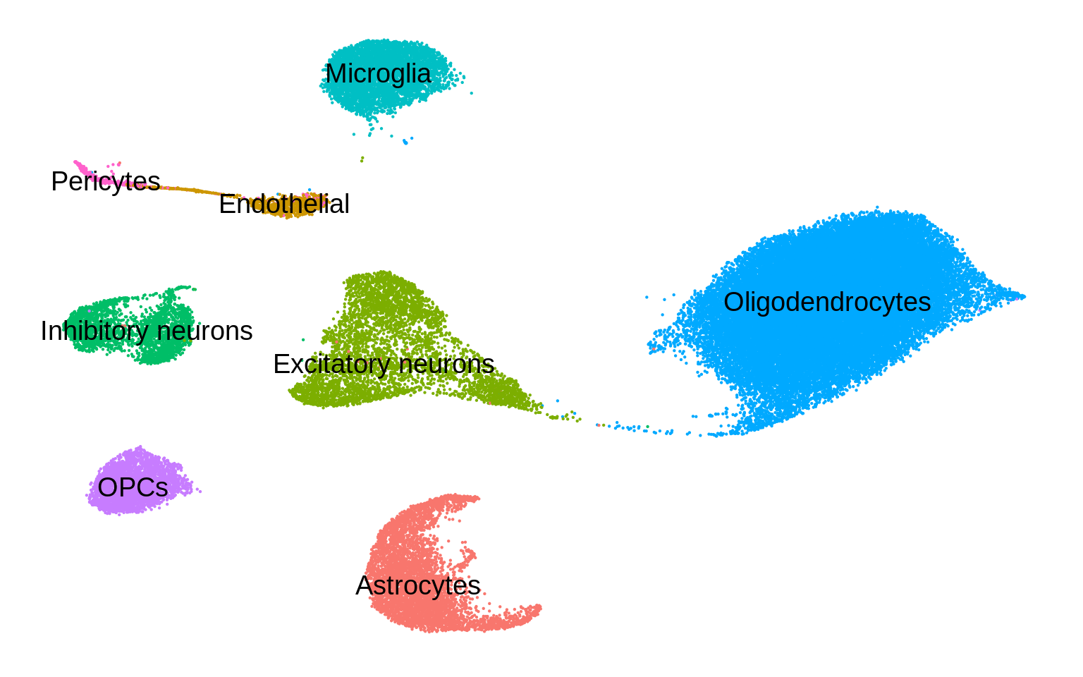
UMAP
umap <- read_tsv('data/umap/umap.ad.subsample.txt')pos <- umap %>% group_by(broad) %>%
summarise(UMAP_1=median(UMAP_1),
UMAP_2=median(UMAP_2))p <- ggplot(umap,aes(UMAP_1,UMAP_2,col=broad)) +
geom_point(size=0.1) +
theme_classic() +
theme(legend.position='none',
axis.text = element_blank(),
axis.ticks = element_blank(),
axis.title = element_blank(),
axis.line = element_blank())
p + geom_text(data=pos,aes(label=broad),col='black',size=5)
Past versions of unnamed-chunk-6-1.png
Version
Author
Date
bb7b4d3
Julien Bryois
2022-01-28
p <- p + geom_text(data=pos,aes(label=broad),col='black',size=9)
ggsave(p,filename = 'output/figures/Figure1_umap.png',width=12,height=8,dpi = 300)
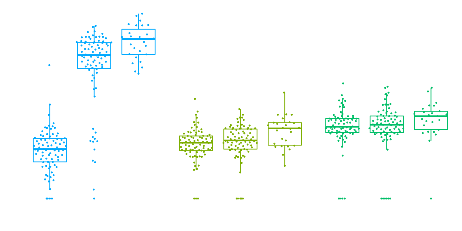
Interaction
hdF5_file_path <- 'output/shiny/data.h5'eqtl_specific <- h5read(hdF5_file_path, "eqtl_results/eqtl_results_specific")plot_eqtl_specific <- function(cell_type_name,gene_name,snp_name,cells_to_display){
gene_short <- gsub('_.+','',gene_name)
genotype <- h5read(hdF5_file_path, paste0("genotype/",snp_name))
expression <- h5read(hdF5_file_path, paste0("expression/",gene_name)) %>%
dplyr::rename(individual=individual_id) %>%
mutate(cell_type=fct_relevel(cell_type,cell_type_name)) %>%
filter(cell_type%in%cells_to_display)
pval <- filter(eqtl_specific,gene==gene_name,cell_type==cell_type_name) %>% pull(nb_pvalue_all_adj)
d <- inner_join(genotype,expression,by='individual') %>%
mutate(genotype_label = case_when(
genotype == 0 ~ paste0(REF,REF),
genotype == 1 ~ paste0(REF,ALT),
genotype == 2 ~ paste0(ALT,ALT)
))
p <- ggplot(d, aes(genotype_label,log2_cpm,col=cell_type)) +
ggbeeswarm::geom_quasirandom(size=0.5) +
geom_boxplot(alpha=0.05,aes(group=genotype_label),outlier.shape = NA) +
theme_classic() +
theme(legend.position='none',text=element_blank(),strip.background = element_blank(),
strip.text.x = element_blank(),axis.text = element_blank(),axis.ticks = element_blank(), axis.line = element_blank()) +
xlab('') +
ylab('') +
facet_wrap(~cell_type,ncol=4) +
scale_color_discrete(limits=levels(d$cell_type) %>% as.character() %>% sort(),drop=FALSE)
p
}gene_name <- 'CHRM5_ENSG00000184984'
snp_name <- 'rs8038713'
cell_type_name <- 'Oligodendrocytes'
cells_to_display <- c('Oligodendrocytes','Excitatory neurons', 'Inhibitory neurons')
chrm5 <- plot_eqtl_specific(cell_type_name,gene_name,snp_name,cells_to_display) + theme(text=element_text(size=20),plot.title = element_text(size=12))
chrm5
Past versions of unnamed-chunk-10-1.png
Version
Author
Date
bb7b4d3
Julien Bryois
2022-01-28
ggsave(chrm5,filename = 'output/figures/Figure1_int.png',width=7,height=3)
Figure 2C
get_snp_pvalues_metabrain <- function(df,chr,tissue='Cortex') {

  write(chr,'metabrain_chr.txt',append=TRUE)
  message(chr)
  d_sig_chr <- filter(df,chr_hg38==chr)

  matched <-
    data.table::fread(paste0('data/metabrain/2020-05-26-',tissue,'-EUR-',chr,'-biogenformat.txt.gz'),data.table = FALSE) %>%
    dplyr::select(p_metabrain=PValue,SNPChr,SNPChrPos,ProbeName,AlleleAssessed,beta_metabrain=`Meta-Beta`,se_metabrain=`Meta-SE`) %>%
    mutate(ensembl=gsub('\\..+','',ProbeName)) %>%
    mutate(SNP_id_hg38=paste0('chr',SNPChr,':',SNPChrPos)) %>%
    as_tibble() %>%
    mutate(tissue=tissue) %>%
    dplyr::select(SNP_id_hg38,ensembl,AlleleAssessed,beta_metabrain,se_metabrain,p_metabrain) %>%
    inner_join(.,d_sig_chr,by=c('SNP_id_hg38','ensembl')) %>%
    filter(AlleleAssessed==effect_allele | AlleleAssessed==other_allele) %>%
    mutate(beta_metabrain=ifelse(AlleleAssessed==effect_allele,beta_metabrain,-beta_metabrain))

  return(matched)
}
d <- read_tsv('output/eqtl/eqtl.PC70.txt') %>%
mutate(se=abs(slope/qnorm(bpval/2))) %>% #compute standard error from pvalue and beta
dplyr::select(cell_type,pid,sid,slope,se,bpval,adj_p) %>%
dplyr::rename(SNP=sid) %>%
separate(pid,into=c('symbol','ensembl'),sep='_')cd data_sensitive/genotypes/processed
zcat combined_final.vcf.gz | cut -f 1,2,3 | grep -v "^#" > snp_pos_hg38.txtsnp_alleles <- data.table::fread('data_sensitive/genotypes/processed/plink.frq',data.table=FALSE) %>% dplyr::select(SNP,effect_allele=A1,other_allele=A2) %>% as_tibble()snp_pos <- data.table::fread('data_sensitive/genotypes/processed/snp_pos_hg38.txt',data.table=FALSE) %>% dplyr::select(SNP=V3,pos_hg38=V2,chr_hg38=V1) %>% as_tibble()d <- left_join(d,snp_alleles,by='SNP') %>%
left_join(.,snp_pos,by='SNP') %>%
mutate(SNP_id_hg38=paste0('chr',chr_hg38,':',pos_hg38)) %>%
dplyr::select(cell_type,symbol,ensembl,SNP,chr_hg38,SNP_id_hg38,effect_allele,other_allele,slope,se,bpval,adj_p)sig <- d %>% filter(adj_p<0.05)
null <- d %>% filter(bpval>0.5)if(!file.exists('output/eqtl/eqtl.PC70.metabrain.matched.txt')){
matched_snps <- lapply(1:22,get_snp_pvalues_metabrain,df=sig) %>%
bind_rows() %>%
group_by(cell_type) %>%
mutate(p_rep_adj=p.adjust(p_metabrain,method='fdr')) %>%
mutate(Replication=ifelse(p_rep_adj<0.05,'5% FDR','Not significant'))
write_tsv(matched_snps,'output/eqtl/eqtl.PC70.metabrain.matched.txt')
} else{
matched_snps <- read_tsv('output/eqtl/eqtl.PC70.metabrain.matched.txt')
}Parsed with column specification:
cols(
SNP_id_hg38 = col_character(),
ensembl = col_character(),
AlleleAssessed = col_character(),
beta_metabrain = col_double(),
se_metabrain = col_double(),
p_metabrain = col_double(),
cell_type = col_character(),
symbol = col_character(),
SNP = col_character(),
chr_hg38 = col_double(),
effect_allele = col_character(),
other_allele = col_character(),
slope = col_double(),
se = col_double(),
bpval = col_double(),
adj_p = col_double(),
p_rep_adj = col_double(),
Replication = col_character()
)if(!file.exists('output/eqtl/eqtl.PC70.metabrain.matched.null.txt')){
null_snps <- lapply(1:22,get_snp_pvalues_metabrain,df=null) %>%
bind_rows()
write_tsv(null_snps,'output/eqtl/eqtl.PC70.metabrain.matched.null.txt')
} else{
null_snps <- read_tsv('output/eqtl/eqtl.PC70.metabrain.matched.null.txt')
}Parsed with column specification:
cols(
SNP_id_hg38 = col_character(),
ensembl = col_character(),
AlleleAssessed = col_character(),
beta_metabrain = col_double(),
se_metabrain = col_double(),
p_metabrain = col_double(),
cell_type = col_character(),
symbol = col_character(),
SNP = col_character(),
chr_hg38 = col_double(),
effect_allele = col_character(),
other_allele = col_character(),
slope = col_double(),
se = col_double(),
bpval = col_double(),
adj_p = col_double()
)matched_snps <- matched_snps %>% mutate(glia_neurons=case_when(
cell_type %in% c('Excitatory neurons','Inhibitory neurons') ~ 'Neurons',
TRUE ~ 'Glia'
)) matched_snps_text <- matched_snps %>%
group_by(glia_neurons) %>%
summarise(n_rep=sum(p_rep_adj < 0.05),
n_rep_same_direction=sum(p_rep_adj < 0.05 & sign(beta_metabrain)==sign(slope)),
n_tot=n(),
prop_rep=n_rep/n_tot,
prop_rep_same_direction=n_rep_same_direction/n_tot,
prop_rep_same_direction_rep=prop_rep_same_direction/prop_rep,
pi1=ifelse(n()>100,round(1-qvalue::qvalue(p_metabrain)$pi0,digits=2),NA)
) %>%
mutate(p1_label=paste0('Pi1 = ', pi1),
prop_rep_label=paste0('5% FDR = ', round(prop_rep*100,digits=0),'%'),
prop_rep_same_label=paste0('Same direction = ', round(prop_rep_same_direction_rep*100,digits=0),'%'),
label=paste0(prop_rep_label,'\n',prop_rep_same_label,'\n',p1_label)
) %>%
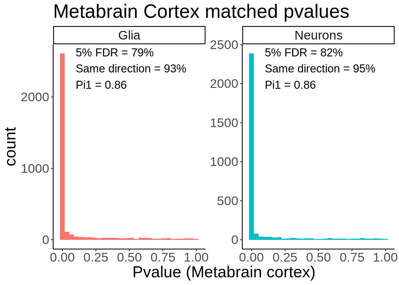
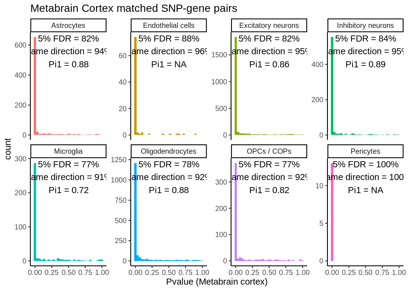
ungroup()`summarise()` ungrouping output (override with `.groups` argument)p <- ggplot(matched_snps,aes(p_metabrain,fill=glia_neurons)) +
geom_histogram() +
facet_wrap(~glia_neurons,scales='free_y') +
theme_classic() +
theme(legend.position = 'none',text=element_text(size=20)) +
geom_text(data=matched_snps_text,aes(x=0.1,y=Inf,vjust=1.1,label=label),size=5,hjust = 0) +
ggtitle('Metabrain Cortex matched pvalues') +
xlab('Pvalue (Metabrain cortex)')
ggsave(p,filename='output/figures/Figure2C.png',height=5,width=7,dpi = 300)
p
Past versions of unnamed-chunk-28-1.png
Version
Author
Date
865a38a
Julien Bryois
2022-02-10
7246d60
Julien Bryois
2022-02-10
Figure 2E
d <- read_tsv('output/eqtl/eqtl.PC70.txt')
d_pb <- read_tsv('output/eqtl/eqtl.pb.PC70.txt') %>%
  dplyr::select(pid,adj_p_pb=adj_p) %>%
  separate(pid,into=c('symbol','ensembl'),sep='_')
loeuf <- read_tsv('data/gnomad_loeuf/supplementary_dataset_11_full_constraint_metrics.tsv') %>%
filter(canonical==TRUE) %>%
dplyr::select(gene,gene_id,transcript,oe_lof_upper,p) %>%
mutate(oe_lof_upper_bin = ntile(oe_lof_upper, 10)) %>%
dplyr::rename(ensembl=gene_id) %>%
dplyr::select(-gene,-transcript)d_loeuf <- d %>%
separate(pid,into=c('symbol','ensembl'),sep='_') %>%
left_join(.,loeuf,by='ensembl') %>%
filter(!is.na(oe_lof_upper))d_loeuf <- inner_join(d_loeuf,d_pb,by=c('ensembl','symbol')) %>%
mutate(Significant=factor(case_when(
adj_p<0.05 & adj_p_pb <0.05 ~ "Both",
adj_p<0.05 & adj_p_pb >=0.05 ~ "Cell",
adj_p>=0.05 & adj_p_pb <0.05 ~ "Bulk",
adj_p>=0.05 & adj_p_pb >=0.05 ~ "None"),
levels=c('None','Cell','Bulk','Both')))my_comparisons <- list( c("None","Cell"),
c("Cell","Bulk"),
c("Bulk","Both"),
c("None","Bulk"),
c("None","Both")
)By Glia vs Neurons
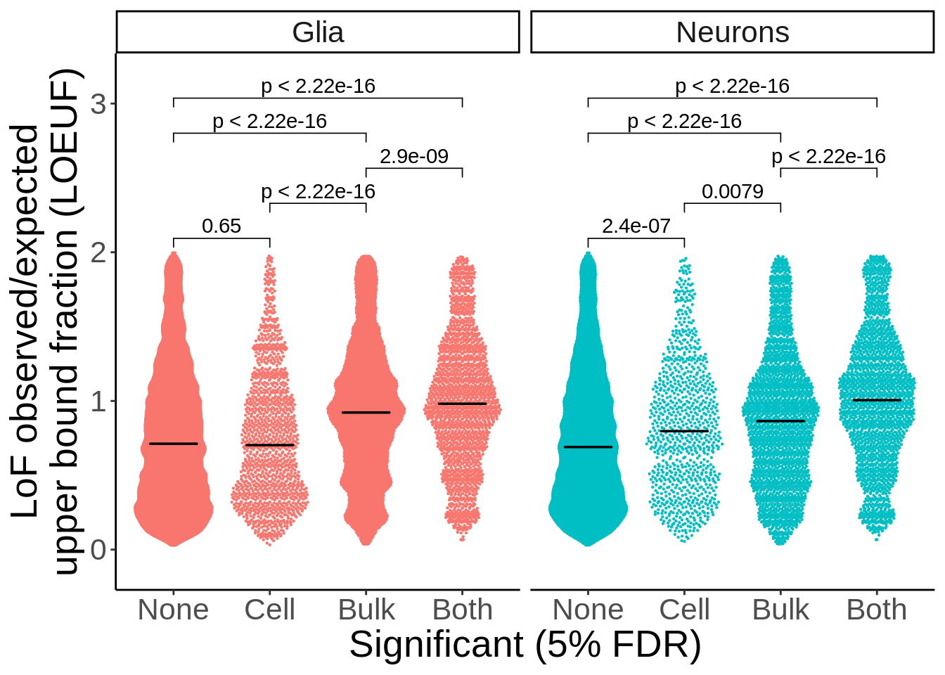
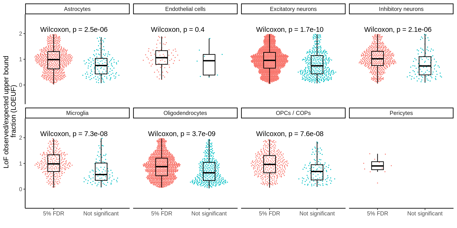
d_loeuf_short <- d_loeuf %>% mutate(type=ifelse(grepl('neurons',cell_type),'Neurons','Glia'))p <- d_loeuf_short %>%
ggplot(.,aes(Significant,oe_lof_upper,col=type)) +
ggbeeswarm::geom_quasirandom(size=0.1) +
facet_wrap(~type,ncol=2) +
theme_classic() +
theme(legend.position='none',text=element_text(size=20)) +
stat_summary(fun = median, fun.min = median, fun.max = median,
geom = "crossbar", width = 0.5,size=0.25,color='black') + xlab("Significant (5% FDR)") + ylab("LoF observed/expected\nupper bound fraction (LOEUF)") +
ggpubr::stat_compare_means(comparisons = my_comparisons) +
scale_y_continuous(expand=c(0.1,0))
ggsave(p,filename='output/figures/Figure2E.png',width = 7,height=5,dpi = 300)
p
Past versions of unnamed-chunk-36-1.png
Version
Author
Date
7246d60
Julien Bryois
2022-02-10
056f5c7
Julien Bryois
2021-12-01
811141f
Julien Bryois
2021-12-01
Figure 2F
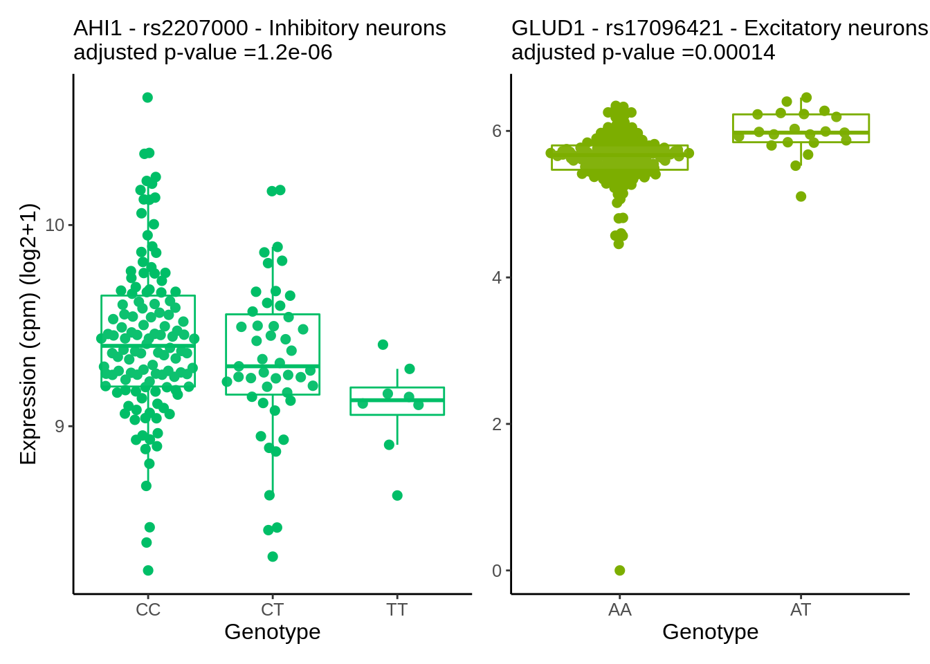
hdF5_file_path <- 'output/shiny/data.h5'eqtl <- h5read(hdF5_file_path, "eqtl_results/eqtl_results_all")plot_eqtl <- function(cell_type_name,gene_name,snp_name,col_point){
gene_short <- gsub('_.+','',gene_name)
genotype <- h5read(hdF5_file_path, paste0("genotype/",snp_name))
expression <- h5read(hdF5_file_path, paste0("expression/",gene_name)) %>%
dplyr::rename(individual=individual_id)
pval <- filter(eqtl,gene==gene_name,cell_type==cell_type_name) %>% pull(adj_p)
d <- inner_join(genotype,expression,by='individual') %>%
mutate(genotype_label = factor(case_when(
genotype == 0 ~ paste0(REF,REF),
genotype == 1 ~ paste0(REF,ALT),
genotype == 2 ~ paste0(ALT,ALT)
),levels=c(unique(paste0(REF,REF)),unique(paste0(REF,ALT)),unique(paste0(ALT,ALT))))) %>% filter(cell_type%in%cell_type_name)
#Only display points for genotypes with more than one individual
n_genotypes <- d %>% dplyr::count(genotype_label) %>%
filter(n>1)
d <- filter(d,genotype_label%in%n_genotypes$genotype_label)
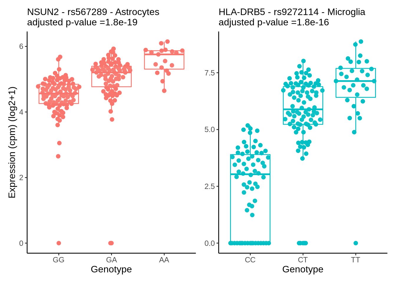
p <- ggplot(d, aes(genotype_label,log2_cpm)) +
ggbeeswarm::geom_quasirandom(size=2,col=col_point) +
geom_boxplot(alpha=0.05,aes(group=genotype_label),outlier.shape = NA,col=col_point) +
theme_classic() +
theme(legend.position='none',text=element_text(size=16), plot.title = element_text(size=10)) +
xlab('Genotype') +
ylab('Expression (cpm) (log2+1)') +
ggtitle(paste0(gene_short,' - ',snp_name,' - ',cell_type_name,'\nadjusted p-value =',signif(pval,digits=2)))
p
}gene_name <- 'HLA-DRB5_ENSG00000198502'
snp_name <- 'rs9272114'
cell_type_name <- 'Microglia'hla <- plot_eqtl(cell_type_name,gene_name,snp_name,'#00BFC4') + theme(axis.title.y = element_blank())gene_name <- 'NSUN2_ENSG00000037474'
snp_name <- 'rs567289'
cell_type_name <- 'Astrocytes'nsun2 <- plot_eqtl(cell_type_name,gene_name,snp_name,'#F8766D')p <- nsun2 + hla & theme(text=element_text(size=24),plot.title = element_text(size=20))
p & theme(text=element_text(size=12),plot.title = element_text(size=12))
Past versions of unnamed-chunk-44-1.png
Version
Author
Date
865a38a
Julien Bryois
2022-02-10
7246d60
Julien Bryois
2022-02-10
f999a54
Julien Bryois
2022-02-02
bb7b4d3
Julien Bryois
2022-01-28
ggsave(p,filename = 'output/figures/Figure2F.png',width=12,height=5)
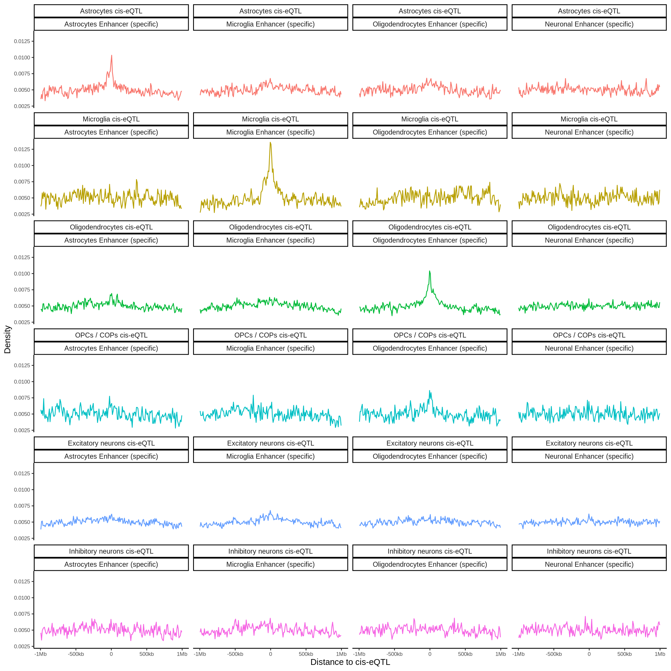
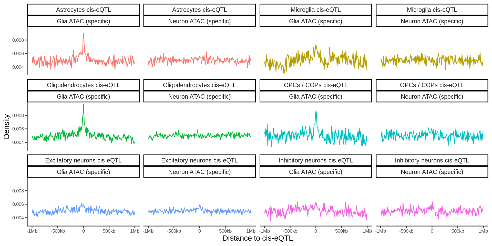
Figure 3A
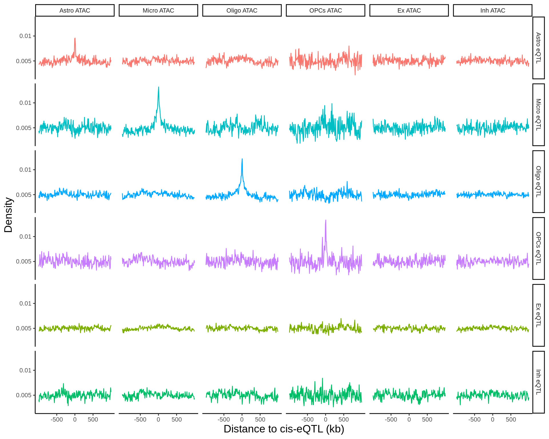
fdensity_files <- list.files('data/epigenome_enrichment/fdensity/results/corces/',full.names = TRUE)fdensity_res <- tibble(fdensity_files) %>% mutate(file_content=map(fdensity_files,read_delim,delim=' ',col_names=FALSE)) %>%
unnest(file_content) %>%
mutate(name=basename(fdensity_files)) %>%
dplyr::select(-fdensity_files) %>%
separate(name,into=c('tmp','sig','annot'),sep='_') %>%
dplyr::select(-tmp) %>%
mutate(sig=gsub('.sig5FDR.bed','',sig)) %>%
mutate(annot=gsub('.bed','',annot)) %>%
group_by(sig,annot) %>%
mutate(X3_norm=X3/sum(X3)) %>%
mutate(sig=gsub('\\.',' ',sig) %>% gsub('OPCs COPs','OPCs / COPs',.)) %>%
mutate(annot=gsub('\\.',' ',annot)) %>%
mutate(annot=gsub(' corces','',annot)) %>%
mutate(annot=gsub('ExcitatoryNeurons','Excitatory neurons',annot)) %>%
mutate(annot=gsub('InhibitoryNeurons','Inhibitory neurons',annot)) %>%
mutate(annot=gsub('OPCs','OPCs / COPs',annot)) %>%
mutate(annot=gsub('specific','ATAC (specific)',annot)) %>%
mutate(sig=paste0(sig,' eQTL')) %>%
mutate(sig=factor(case_when(
sig=='Astrocytes eQTL' ~ 'Astro eQTL',
sig=='Endothelial cells eQTL' ~ 'Endo eQTL',
sig=='Excitatory neurons eQTL' ~ 'Ex eQTL',
sig=='Inhibitory neurons eQTL' ~ 'Inh eQTL',
sig=='Microglia eQTL' ~ 'Micro eQTL',
sig=='Oligodendrocytes eQTL' ~ 'Oligo eQTL',
sig=='OPCs / COPs eQTL' ~ 'OPCs eQTL',
sig=='Pericytes eQTL' ~ 'Pericytes eQTL'),
levels=c('Astro eQTL','Micro eQTL','Oligo eQTL','OPCs eQTL','Ex eQTL','Inh eQTL','Endo eQTL','Pericytes eQTL'))) %>%
filter(grepl('ATAC',annot)) %>%
mutate(annot=factor(case_when(
annot=='Astrocytes ATAC (specific)' ~ 'Astro ATAC',
annot=='Excitatory neurons ATAC (specific)' ~ 'Ex ATAC',
annot=='Inhibitory neurons ATAC (specific)' ~ 'Inh ATAC',
annot=='Microglia ATAC (specific)' ~ 'Micro ATAC',
annot=='Oligodendrocytes ATAC (specific)' ~ 'Oligo ATAC',
annot=='OPCs / COPs ATAC (specific)' ~ 'OPCs ATAC'),levels=c('Astro ATAC','Micro ATAC','Oligo ATAC','OPCs ATAC','Ex ATAC','Inh ATAC')))cols <- scales::hue_pal()(8)[c(1,5,6,7,3,4)]
p <- fdensity_res %>% filter(!sig%in%c('Pericytes eQTL','Endo eQTL'),grepl('ATAC',annot)) %>% ggplot(.,aes((X1+X2)/2,X3_norm,col=sig)) + geom_line() + facet_grid(sig~annot) + theme_classic() + theme(legend.position = 'none',text=element_text(size=18),axis.title = element_text(size=30)) + xlab('Distance to cis-eQTL (kb)') + ylab('Density') + scale_x_continuous(breaks=c(-500000,0,500000),labels = c('-500','0','500')) + scale_y_continuous(breaks=c(0.005,0.010,0.015),labels = c('0.005','0.01','0.015')) + scale_color_manual(values=cols)
ggsave(p,filename = 'output/figures/Figure3A.png',width=11,height=8.5,dpi = 300)
p + theme(text=element_text(size=10),axis.title = element_text(size=14))
Past versions of unnamed-chunk-52-1.png
Version
Author
Date
7246d60
Julien Bryois
2022-02-10
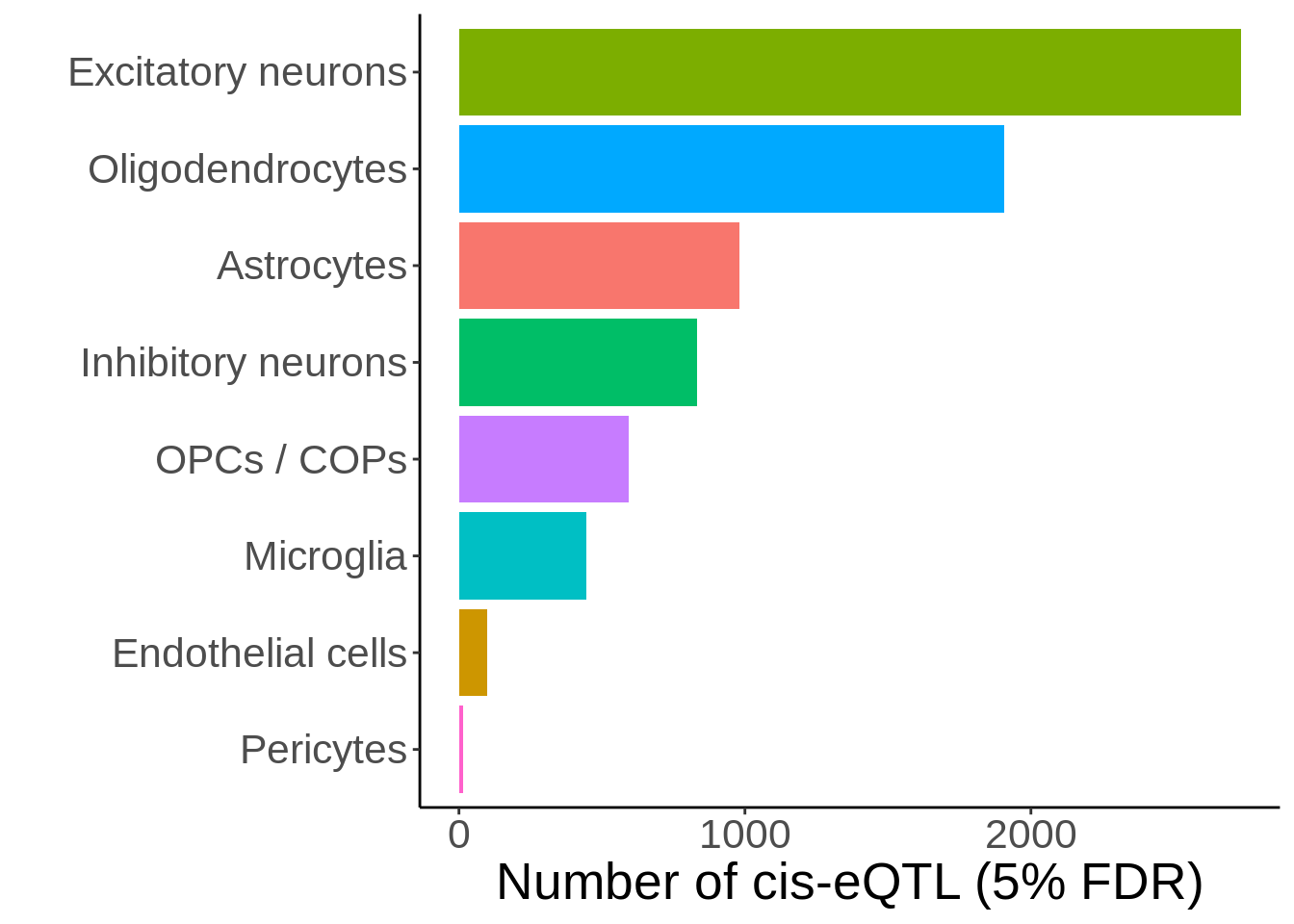
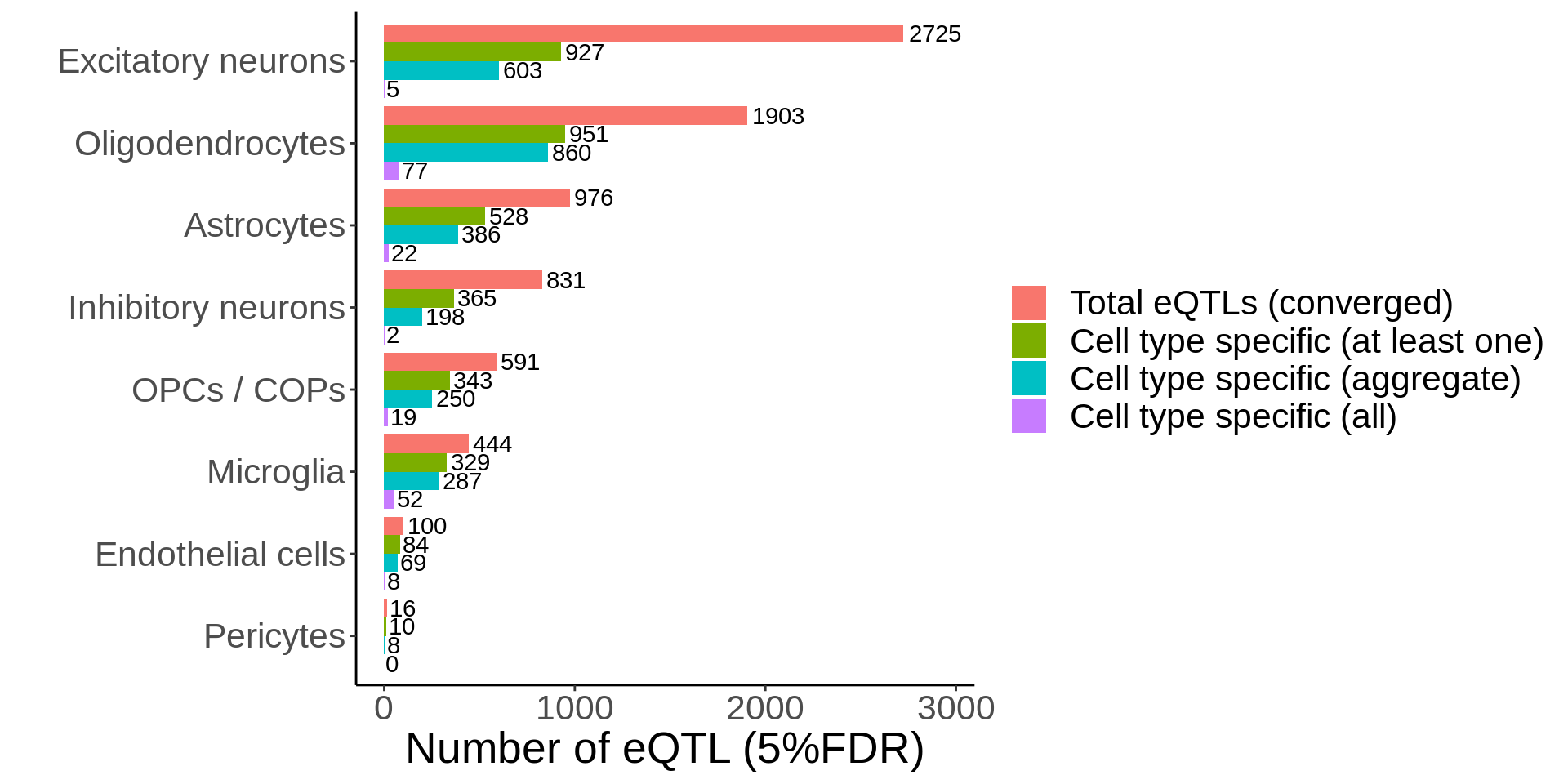
Figure 3B
d <- read_tsv('output/eqtl_specific/eqtl.PC70.specific.txt') %>%
#Sets pvalue to NA if the model did not converge
mutate(nb_pvalue_aggregate=ifelse(nb_pvalue_aggregate_model_converged==FALSE,NA,nb_pvalue_aggregate)) %>%
mutate(nb_pvalue_at_least_one=ifelse(nb_pvalue_at_least_one_model_converged==FALSE,NA,nb_pvalue_at_least_one)) %>% #Remove genes for which the model did not converge (9 genes)
filter(!is.na(nb_pvalue_aggregate),
!is.na(nb_pvalue_at_least_one),
nb_pvalue_at_least_one!=Inf) %>%
#Get adjusted pvalues
mutate(nb_pvalue_aggregate_adj=p.adjust(nb_pvalue_aggregate,method='fdr'),
nb_pvalue_at_least_one_adj=p.adjust(nb_pvalue_at_least_one,method = 'fdr')) %>%
#For each row, get the maximum pvalue across all cell types, this will be the gene-level pvalue testing whether the genetic effect on gene expression is different than all other cell types
rowwise() %>%
mutate(nb_pvalue_sig_all=max(Astrocytes_p,`Endothelial cells_p`,`Excitatory neurons_p`,`Inhibitory neurons_p`,Microglia_p,Oligodendrocytes_p,`OPCs / COPs_p`,Pericytes_p,na.rm=TRUE)) %>%
ungroup() %>%
mutate(nb_pvalue_all_adj = p.adjust(nb_pvalue_sig_all,method='fdr'))d_short <- d %>%
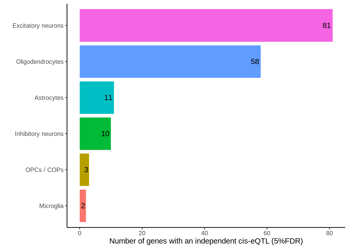
dplyr::select(cell_type_id,gene_id,snp_id,nb_pvalue_aggregate_adj,nb_pvalue_at_least_one_adj,nb_pvalue_all_adj)p <- d_short %>% ungroup() %>%
group_by(cell_type_id) %>%
summarise(
`Cell type specific (aggregate)`=sum(nb_pvalue_aggregate_adj<0.05,na.rm=TRUE),
`Cell type specific (at least one)`=sum(nb_pvalue_at_least_one_adj<0.05,na.rm=TRUE),
`Cell type specific (all)`=sum(nb_pvalue_all_adj<0.05),
`Total eQTLs (converged)`=n()) %>%
tidyr::gather(type,value,-cell_type_id) %>%
mutate(type=factor(type,levels=rev(c('Total eQTLs (converged)','Cell type specific (at least one)','Cell type specific (aggregate)','Cell type specific (all)')))) %>%
mutate(cell_type_id=factor(cell_type_id,levels=rev(c('Excitatory neurons','Oligodendrocytes','Astrocytes','Inhibitory neurons','OPCs / COPs','Microglia','Endothelial cells','Pericytes')))) %>%
ggplot(.,aes(value,cell_type_id,fill=type)) +
geom_col(position = position_dodge()) +
guides(fill = guide_legend(reverse = TRUE)) +
geom_text(aes(label=value),position = position_dodge(width = 0.9),hjust=-0.1) +
xlim(c(0,2950)) +
ylab('') +
theme_classic() +
xlab('Number of eQTL (5%FDR)') +
scale_fill_hue(direction = -1) +
theme(legend.position='right', text=element_text(size=20),legend.title = element_blank())
ggsave(p,filename='output/figures/Figure3B.png',height=6,width=13,dpi = 300)
p
Past versions of unnamed-chunk-55-1.png
Version
Author
Date
865a38a
Julien Bryois
2022-02-10
7246d60
Julien Bryois
2022-02-10
Figure 3C
d <- read_tsv('output/eqtl_specific/eqtl.PC70.specific.txt') %>%
#Sets pvalue to NA if the model did not converge
mutate(nb_pvalue_aggregate=ifelse(nb_pvalue_aggregate_model_converged==FALSE,NA,nb_pvalue_aggregate)) %>%
mutate(nb_pvalue_at_least_one=ifelse(nb_pvalue_at_least_one_model_converged==FALSE,NA,nb_pvalue_at_least_one)) %>% #Remove genes for which the model did not converge (9 genes)
filter(!is.na(nb_pvalue_aggregate),
!is.na(nb_pvalue_at_least_one),
nb_pvalue_at_least_one!=Inf)d_gather <- d %>%
dplyr::select(-snp_id) %>%
gather(cell_type_test,p,-cell_type_id,-gene_id,-nb_pvalue_aggregate,-nb_pvalue_at_least_one,-nb_pvalue_aggregate_model_converged,-nb_pvalue_at_least_one_model_converged) %>%
mutate(cell_type_test=gsub('_p','',cell_type_test)) %>%
mutate(cell_type_id=factor(cell_type_id,levels=c('Microglia','OPCs / COPs', 'Astrocytes','Oligodendrocytes','Inhibitory neurons', 'Excitatory neurons','Endothelial cells','Pericytes')),
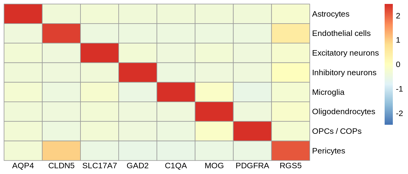
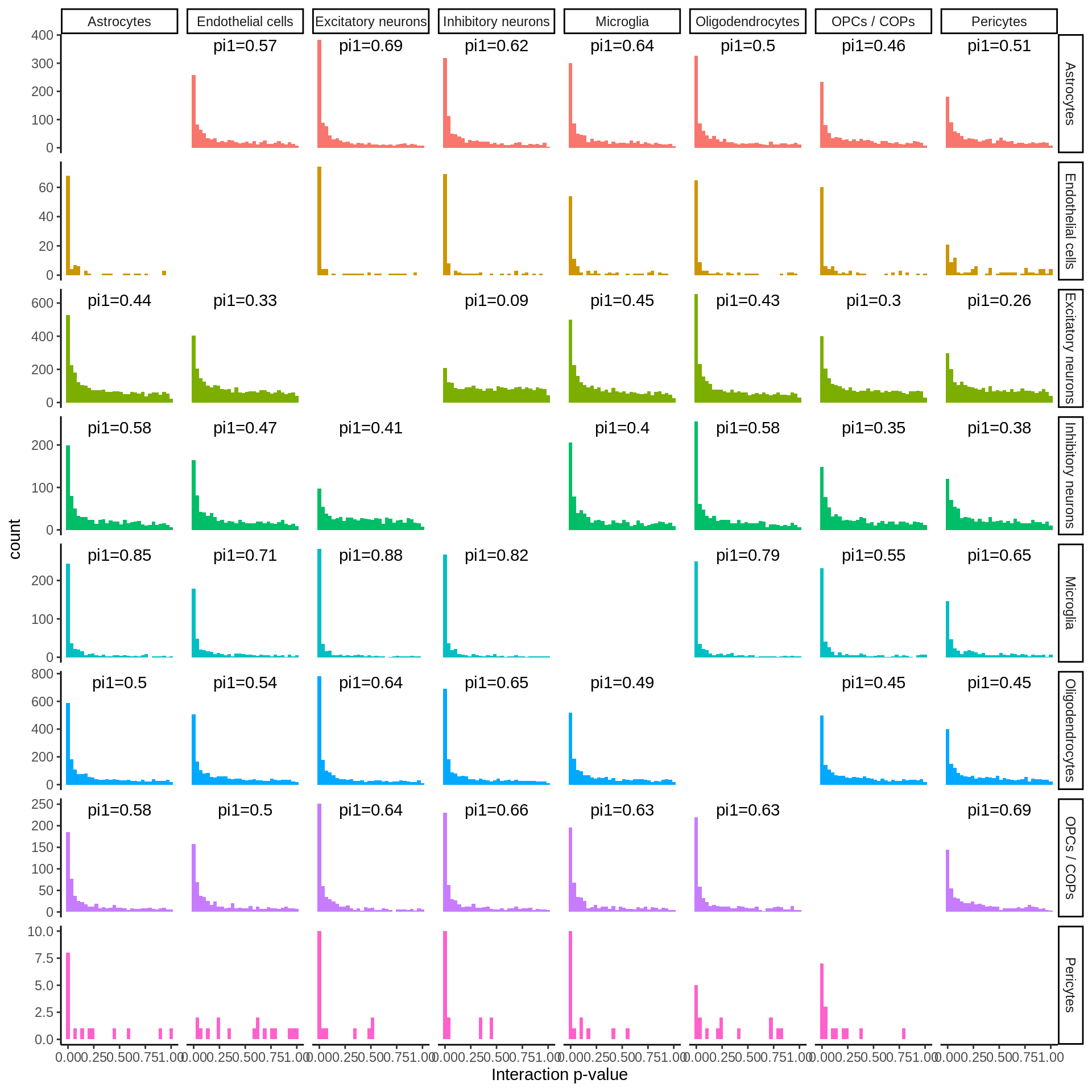
cell_type_test=factor(cell_type_test,levels=c('Microglia','OPCs / COPs', 'Astrocytes','Oligodendrocytes','Inhibitory neurons', 'Excitatory neurons','Endothelial cells','Pericytes')))pi1 <- d_gather %>%
filter(!is.na(p)) %>%
filter(!cell_type_id%in%c('Endothelial cells','Pericytes')) %>%
group_by(cell_type_id,cell_type_test) %>%
summarise(pi1=1-qvalue::qvalue(p)$pi0)pi1 %>% spread(cell_type_test,pi1) %>% column_to_rownames('cell_type_id') %>% pheatmap::pheatmap(.,display_numbers = TRUE,number_color = 'black',angle_col = 45) %>% print()
Past versions of unnamed-chunk-59-1.png
Version
Author
Date
7246d60
Julien Bryois
2022-02-10
f999a54
Julien Bryois
2022-02-02
bb7b4d3
Julien Bryois
2022-01-28
pi1 %>% spread(cell_type_test,pi1) %>% column_to_rownames('cell_type_id') %>% pheatmap::pheatmap(.,display_numbers = TRUE,number_color = 'black',angle_col = 45,filename = 'output/figures/Figure3C.png',height = 4)
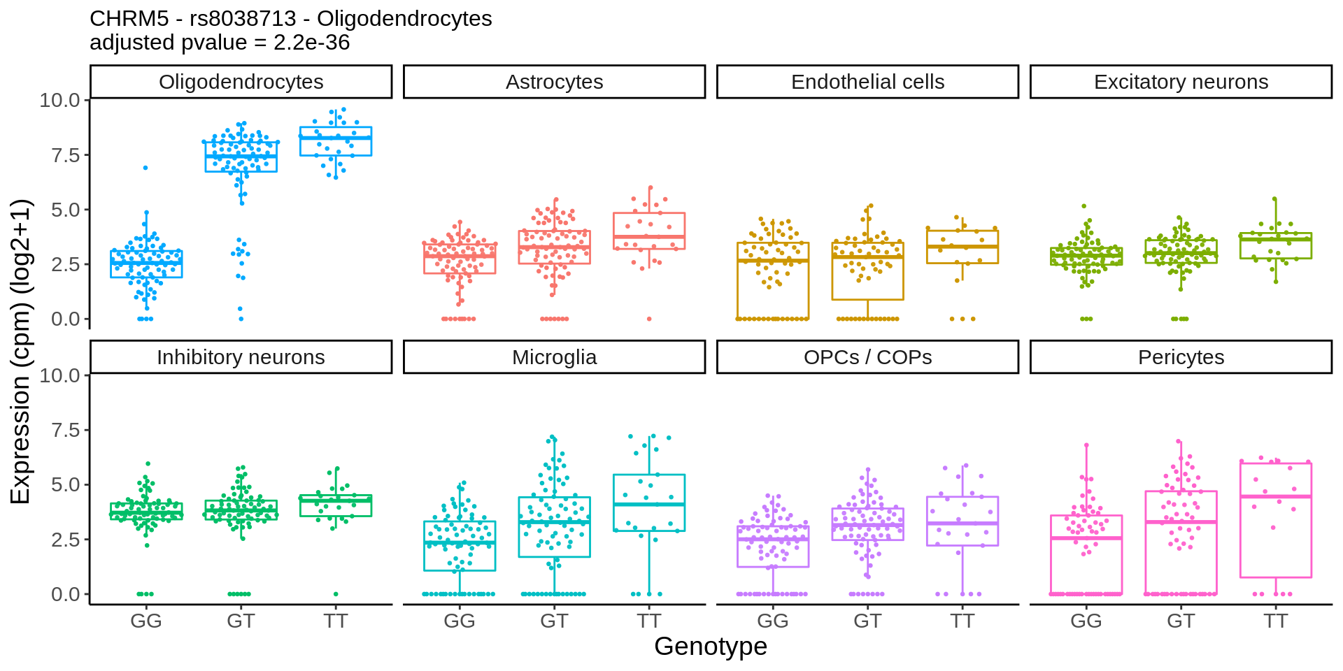
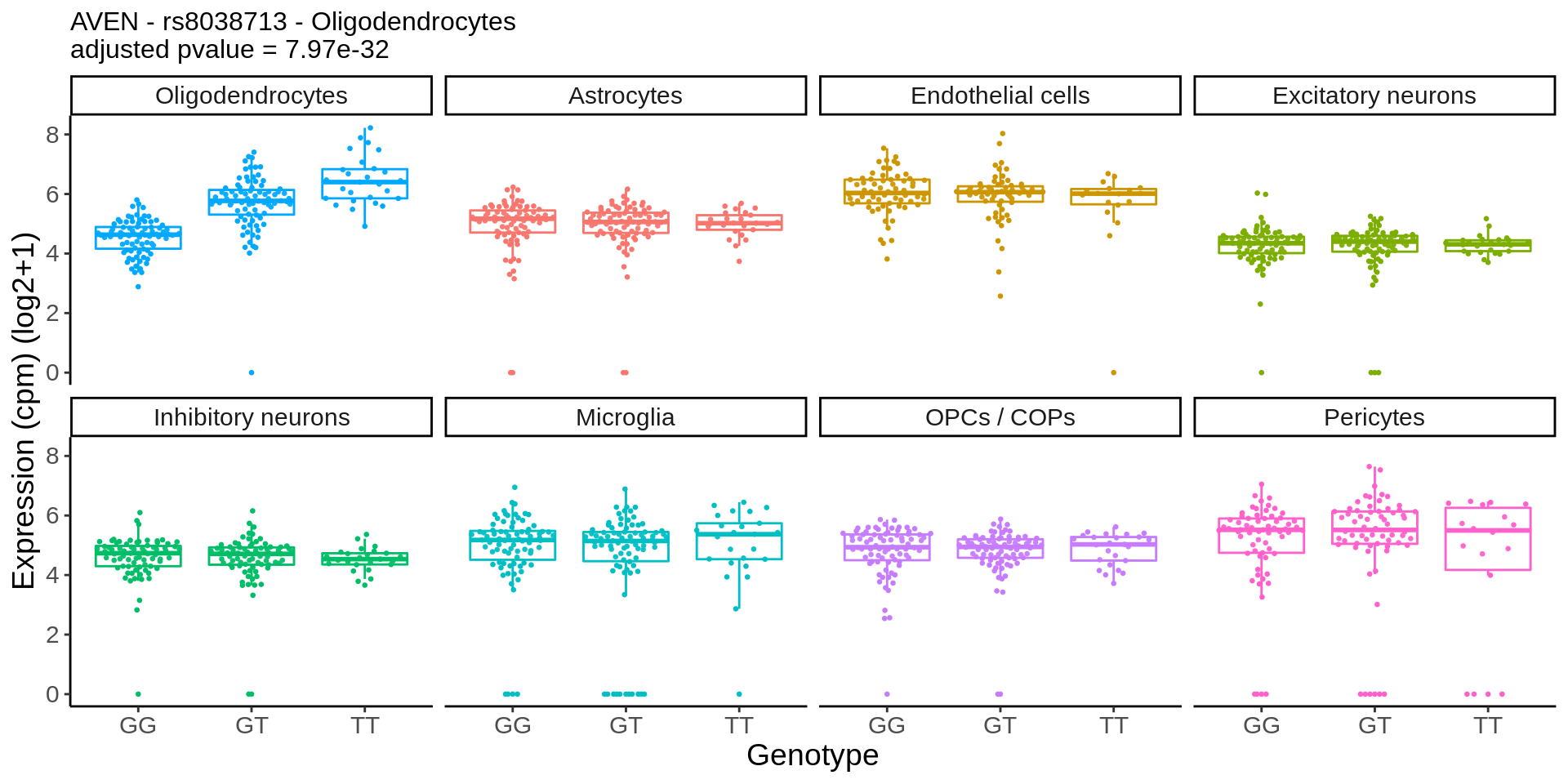
Figure 3D
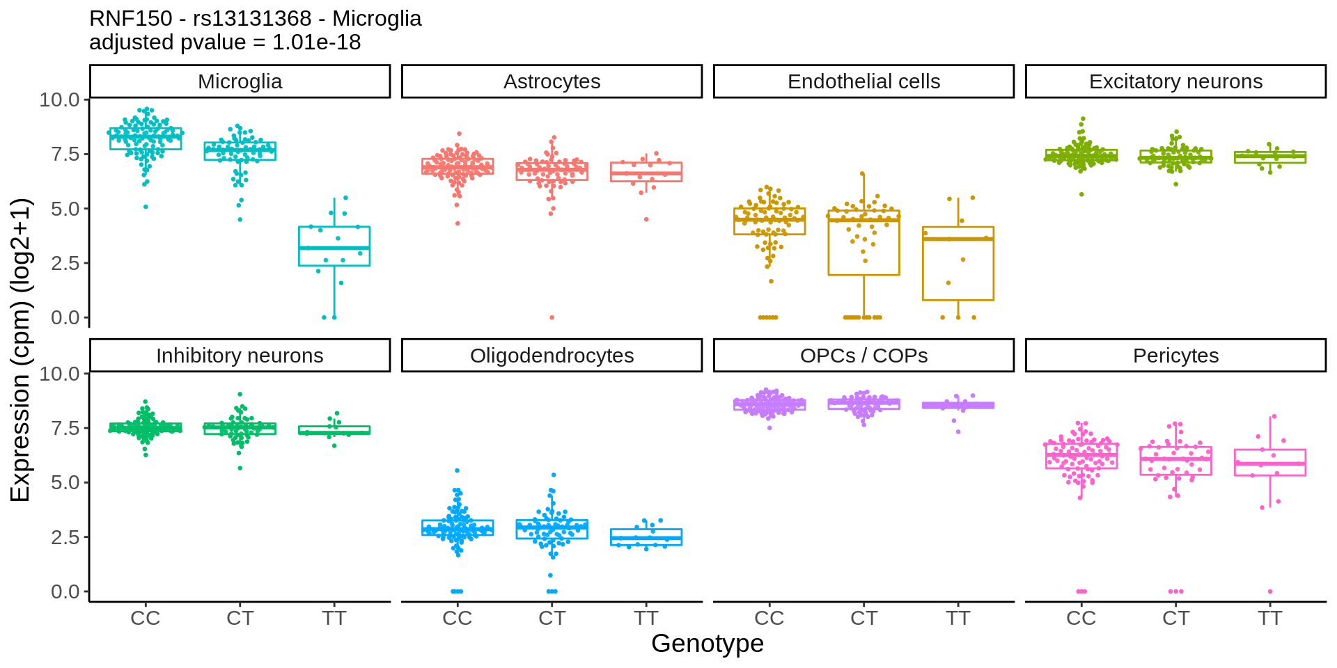
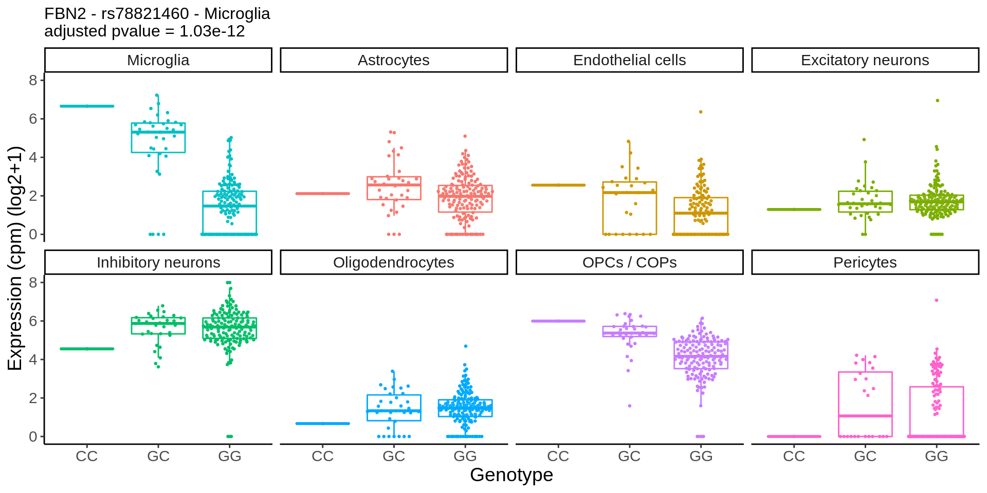
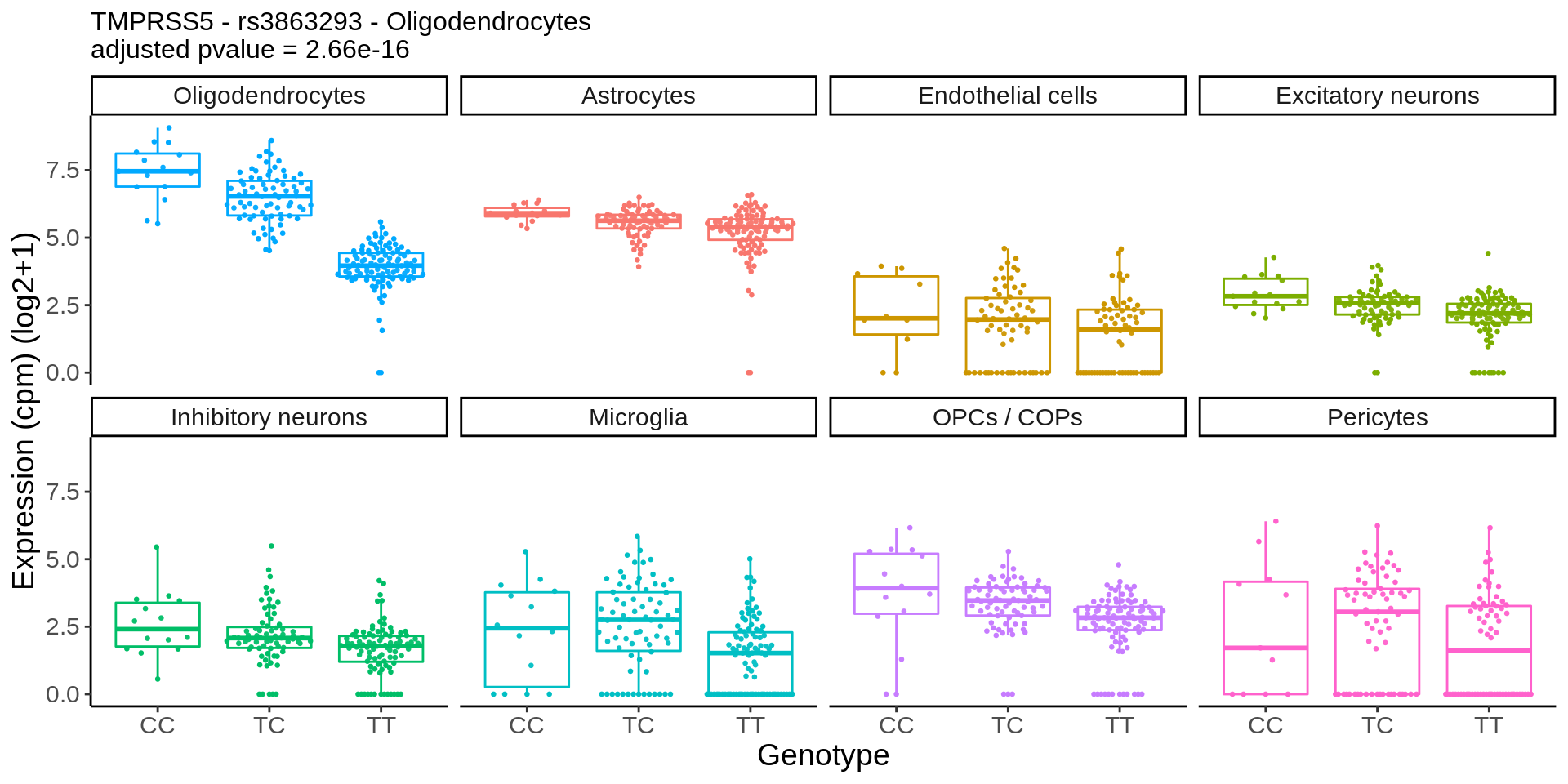
hdF5_file_path <- 'output/shiny/data.h5'eqtl_specific <- h5read(hdF5_file_path, "eqtl_results/eqtl_results_specific")plot_eqtl_specific <- function(cell_type_name,gene_name,snp_name){
gene_short <- gsub('_.+','',gene_name)
genotype <- h5read(hdF5_file_path, paste0("genotype/",snp_name))
expression <- h5read(hdF5_file_path, paste0("expression/",gene_name)) %>%
dplyr::rename(individual=individual_id)
pval <- filter(eqtl_specific,gene==gene_name,cell_type==cell_type_name) %>% pull(nb_pvalue_all_adj)
d <- inner_join(genotype,expression,by='individual') %>%
mutate(genotype_label = case_when(
genotype == 0 ~ paste0(REF,REF),
genotype == 1 ~ paste0(REF,ALT),
genotype == 2 ~ paste0(ALT,ALT)
)) %>% mutate(cell_type=fct_relevel(cell_type,cell_type_name))
p <- ggplot(d, aes(genotype_label,log2_cpm,col=cell_type)) +
ggbeeswarm::geom_quasirandom(size=0.5) +
geom_boxplot(alpha=0.05,aes(group=genotype_label),outlier.shape = NA) +
theme_classic() +
theme(legend.position='none',text=element_text(size=16), plot.title = element_text(size=10)) +
xlab('Genotype') +
ylab('Expression (cpm) (log2+1)') +
ggtitle(paste0(gene_short,' - ',snp_name,' - ',cell_type_name,'\nadjusted pvalue = ', pval)) + facet_wrap(~cell_type,ncol=4) + scale_color_discrete(limits=unique(d$cell_type) %>% as.character() %>% sort())
p
}gene_name <- 'CHRM5_ENSG00000184984'
snp_name <- 'rs8038713'
cell_type_name <- 'Oligodendrocytes'
chrm5 <- plot_eqtl_specific(cell_type_name,gene_name,snp_name) + theme(text=element_text(size=20),plot.title = element_text(size=12))
chrm5 + theme(text=element_text(size=14))
Past versions of unnamed-chunk-64-1.png
Version
Author
Date
865a38a
Julien Bryois
2022-02-10
7246d60
Julien Bryois
2022-02-10
ggsave(chrm5,filename = 'output/figures/Figure3D.png',width=9,height=5)
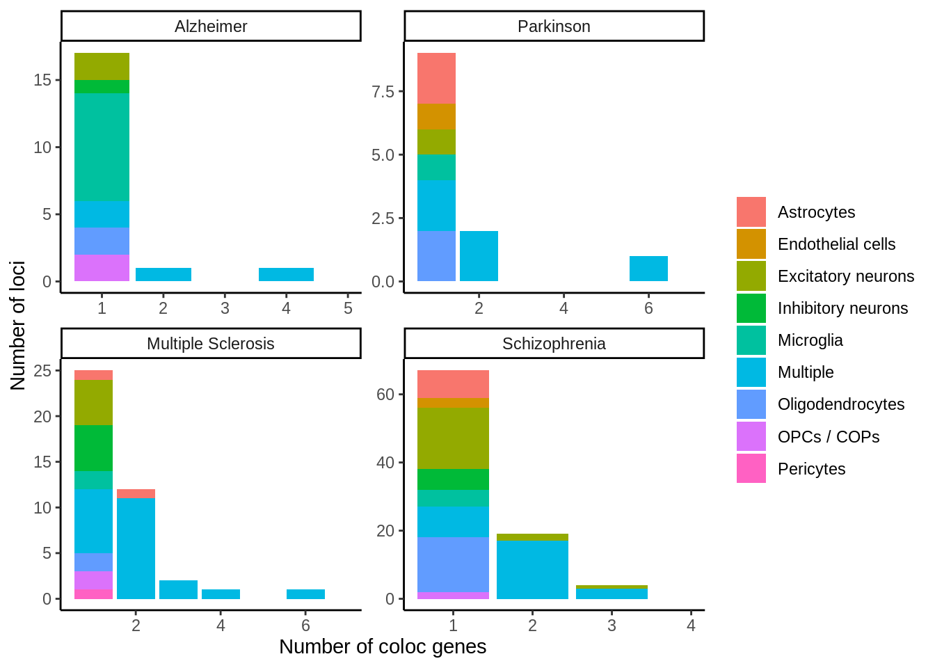
Figure 4A
read_coloc <- function(path){
coloc <- read_tsv(path) %>%
dplyr::select(locus,closest_gene,ensembl,symbol,tissue,PP.H4.abf) %>%
dplyr::rename(phenotype=ensembl,hgnc_symbol=symbol,locus_name=locus)
#If coloc was performed for the same genes located in loci in close proximity, take the best
coloc <- coloc %>% group_by(phenotype,tissue) %>%
slice_max(n=1,order_by=PP.H4.abf,with_ties=FALSE) %>%
ungroup()
return(coloc)
}coloc_ms <- read_coloc('output/coloc/coloc.ms.txt') %>% mutate(trait='Multiple Sclerosis')
coloc_ad <- read_coloc('output/coloc/coloc.ad.txt') %>% mutate(trait='Alzheimer')
coloc_scz <- read_coloc('output/coloc/coloc.scz.txt') %>% mutate(trait='Schizophrenia')
coloc_pd <- read_coloc('output/coloc/coloc.pd.txt') %>% mutate(trait='Parkinson')coloc <- rbind(coloc_ms,coloc_ad,coloc_scz,coloc_pd)my_ceil <- function(x) {
ceil <- ceiling(max(x))
#ifelse(ceil > 1 & ceil %% 2 == 1, ceil + 1, ceil)
}
my_breaks <- function(x) {
ceil <- my_ceil(max(x))
unique(ceiling(pretty(seq(0, ceil))))
}
my_limits <- function(x) {
ceil <- my_ceil(x[2])
c(x[1], ceil)
}x <- coloc %>%
filter(PP.H4.abf>=0.7) %>%
dplyr::select(trait,closest_gene,hgnc_symbol,tissue) %>%
group_by(trait,closest_gene,hgnc_symbol) %>%
mutate(n_cell_types_per_locus=length(unique(tissue))) %>%
ungroup() %>%
group_by(trait,closest_gene) %>%
mutate(n_genes_per_loci=length(unique(hgnc_symbol))) %>%
ungroup() %>%
mutate(cell_type=ifelse(n_cell_types_per_locus>1,'Multiple',tissue)) %>%
dplyr::select(-n_cell_types_per_locus,-tissue) %>%
unique() %>%
group_by(closest_gene) %>%
mutate(n_cell_type=length(unique(cell_type))) %>%
ungroup() %>%
mutate(cell_type2=ifelse(n_cell_type>1,'Multiple',cell_type)) %>%
dplyr::select(trait,closest_gene,hgnc_symbol,n_genes_per_loci,cell_type2) %>%
mutate(trait=factor(trait,levels=c('Alzheimer','Parkinson','Multiple Sclerosis','Schizophrenia'))) %>%
dplyr::select(trait,closest_gene,n_genes_per_loci,cell_type2) %>% unique() %>%
dplyr::count(trait,n_genes_per_loci,cell_type2)p <- ggplot(x,aes(n_genes_per_loci,n,fill=cell_type2)) + geom_col() + facet_wrap(~trait,scales = 'free') + xlab('Number of coloc genes') + ylab('Number of loci') + theme_classic() + scale_x_continuous(breaks=my_breaks,limits=my_limits) + guides(fill=guide_legend(title=''))
p
Past versions of unnamed-chunk-72-1.png
Version
Author
Date
7246d60
Julien Bryois
2022-02-10
p <- p + theme(text=element_text(size=50),axis.ticks.length=unit(.25, "cm"),legend.position='top',legend.text = element_text(size=22))
ggsave(p,filename='output/figures/Figure4A.png',width=16,height=12,dpi = 300)
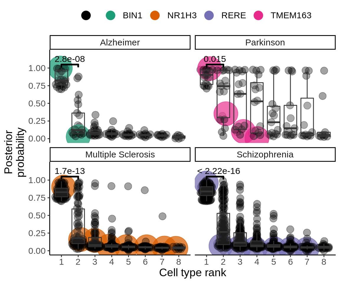
Figure 4B
read_coloc <- function(path){
coloc <- read_tsv(path) %>%
dplyr::select(locus,closest_gene,ensembl,symbol,tissue,PP.H4.abf) %>%
dplyr::rename(phenotype=ensembl,hgnc_symbol=symbol,locus_name=locus)
#If coloc was performed for the same genes located in loci in close proximity, take the best
coloc <- coloc %>% group_by(phenotype,tissue) %>%
slice_max(n=1,order_by=PP.H4.abf,with_ties=FALSE) %>%
ungroup()
return(coloc)
}coloc_ms <- read_coloc('output/coloc/coloc.ms.txt') %>% mutate(trait='Multiple Sclerosis')
coloc_ad <- read_coloc('output/coloc/coloc.ad.txt') %>% mutate(trait='Alzheimer')
coloc_scz <- read_coloc('output/coloc/coloc.scz.txt') %>% mutate(trait='Schizophrenia')
coloc_pd <- read_coloc('output/coloc/coloc.pd.txt') %>% mutate(trait='Parkinson')coloc <- rbind(coloc_ms,coloc_ad,coloc_scz,coloc_pd)genes_with_coloc <- coloc %>%
group_by(trait) %>%
filter(PP.H4.abf>0.7) %>%
dplyr::select(phenotype,trait) %>%
unique()coloc_selected <- coloc %>%
inner_join(.,genes_with_coloc,by=c('phenotype','trait')) %>%
group_by(phenotype,trait) %>%
mutate(rank_coloc=rank(-PP.H4.abf)) %>%
mutate(lab=case_when(
hgnc_symbol=='BIN1' ~ 'BIN1',
hgnc_symbol=='TMEM163' ~ 'TMEM163',
hgnc_symbol=='NR1H3' ~ 'NR1H3',
hgnc_symbol=='RERE' ~ 'RERE',
TRUE ~ ''
)) %>%
mutate(lab_size=case_when(
hgnc_symbol=='BIN1' ~ 8,
hgnc_symbol=='TMEM163' ~ 8,
hgnc_symbol=='NR1H3' ~ 8,
hgnc_symbol=='RERE' ~ 8,
TRUE ~ 4
))my_comparisons <- list( c("1", "2"))
coloc_selected <- mutate(coloc_selected,trait=factor(trait,levels=c('Alzheimer','Parkinson','Multiple Sclerosis','Schizophrenia')))
p <- ggplot(coloc_selected,aes(as.factor(rank_coloc),PP.H4.abf,group=rank_coloc)) +
ggbeeswarm::geom_quasirandom(aes(col=lab,size=lab_size,alpha=lab_size)) +
geom_boxplot(alpha=0.1,outlier.shape = NA) +
facet_wrap(~trait,ncol=2) +
theme_classic() +
xlab('Cell type rank') +
ylab('Posterior\nprobability') +
scale_y_continuous(limits = c(0,1.2),breaks=c(0,0.25,0.5,0.75,1)) +
scale_x_discrete(expand=c(0.1,0)) +
scale_color_manual(values=c('black','#1B9E77','#D95F02','#7570B3','#E7298A')) +
guides(size=FALSE) +
scale_alpha_binned(range = c(0.3,0.8),guide='none') +
theme(legend.position='top',text=element_text(size=48),legend.title = element_blank()) +
guides(colour = guide_legend(override.aes = list(size=10))) +
scale_size_continuous(range = c(4, 14))
p_figure <- p + ggpubr::stat_compare_means(comparisons = my_comparisons,size=10,vjust = -0.3,bracket.size = 1)
ggsave(p_figure,filename='output/figures/Figure4B.png',width=19,height=12,dpi = 300)
p + theme(legend.position='top',text=element_text(size=14),legend.title = element_blank()) +
guides(colour = guide_legend(override.aes = list(size=5))) +
ggpubr::stat_compare_means(comparisons = my_comparisons,size=4,vjust = -0.3,bracket.size = 1)
Past versions of unnamed-chunk-78-1.png
Version
Author
Date
7246d60
Julien Bryois
2022-02-10
Figure 4C
coloc_heatmap <- function(file,threshold=0.7,width=7,height=5,out_name){
coloc_all <- read_tsv(file)
trait <- basename(file) %>% gsub('coloc.','',.) %>% gsub('.txt','',.)
metabrain_s1 <- readxl::read_xlsx('data/metabrain/media-1.xlsx',skip=1,sheet = 2) %>%
mutate(disease=case_when(
outcome=="Alzheimer’s disease" ~ 'ad',
outcome=="Multiple sclerosis" ~ 'ms',
outcome=="Parkinson’s disease" ~ 'pd',
outcome=="Schizophrenia" ~ 'scz',
TRUE ~ outcome
)) %>%
dplyr::select(gene,disease) %>%
filter(disease==trait)
#Get best coloc if same gene in same cell type was tested in two different loci
coloc_all <- coloc_all %>% group_by(ensembl,tissue) %>%
slice_max(n=1,order_by=PP.H4.abf,with_ties=FALSE) %>%
ungroup() %>%
mutate(symbol=ifelse(symbol%in%metabrain_s1$gene,paste0(symbol,'*'),symbol))
#Get best coloc if same symbol in same cell type was tested multiple times (different ensembl name for same symbol at same locus)
coloc_all <- coloc_all %>% group_by(symbol,tissue) %>%
slice_max(n=1,order_by=PP.H4.abf,with_ties=FALSE) %>%
ungroup()
#Get absolute value of effect size of the GWAS
coloc_all <- mutate(coloc_all,beta=abs(beta_top_GWAS))
coloc_all_matrix <- dplyr::select(coloc_all,tissue,symbol,PP.H4.abf) %>%
filter(!is.na(symbol)) %>%
unique() %>%
spread(tissue,PP.H4.abf,fill=0) %>%
column_to_rownames('symbol')
coloc_all_format_per_gene <- coloc_all %>%
group_by(ensembl) %>%
filter(PP.H4.abf==max(PP.H4.abf),PP.H4.abf>threshold) %>%
mutate(closest_gene=gsub('ENSG.+ - | - ENSG.+','',closest_gene)) %>% #Remove ENSEMBL name if a symbol + and ensembl gene name
#are both at same distance from GWAS top pick
ungroup() %>%
dplyr::rename(symbol_coloc=symbol) %>%
filter(!is.na(symbol_coloc)) %>%
arrange(-PP.H4.abf) %>%
mutate(risk=case_when(
direction ==1 ~ 'Up',
direction ==-1 ~ 'Down',
direction ==0 ~ 'Isoform'
)) %>%
column_to_rownames('symbol_coloc') %>%
dplyr::rename(LOEUF=oe_lof_upper_bin)
coloc_all_matrix_subset <- coloc_all_matrix[apply(coloc_all_matrix,1,function(x) any(x>threshold)),] %>% as.matrix()
coloc_all_format_per_gene_direction <- coloc_all_format_per_gene[rownames(coloc_all_matrix_subset),] %>%
dplyr::select(closest_gene,risk,LOEUF,beta)
ha = HeatmapAnnotation(df = coloc_all_format_per_gene_direction[,2:3,drop=FALSE],
which ='row',
col = list('risk' = c("Up"="#E31A1C","Down"="#1F78B4","Isoform"="darkorange"),
'LOEUF' = circlize::colorRamp2(c(0,10),c('white','springgreen4'))),
show_annotation_name = c('risk' = TRUE,'LOEUF'=TRUE),
annotation_name_rot = 45
)
hb = HeatmapAnnotation(df = coloc_all_format_per_gene_direction[,4,drop=FALSE],
which ='row',
col = list(circlize::colorRamp2(c(min(coloc_all_format_per_gene_direction[[4]],na.rm=T),
max(coloc_all_format_per_gene_direction[[4]],na.rm=T)),c('white','palevioletred3'))) %>%
setNames(colnames(coloc_all_format_per_gene_direction)[4]),
annotation_name_rot = 45
)
ht <- Heatmap(coloc_all_matrix_subset,col=viridis(100),
right_annotation=ha,column_names_rot = 45,
left_annotation = hb,
#row_names_side = 'left',
#row_dend_side = 'right',
row_split = coloc_all_format_per_gene_direction[, 1],
row_title_rot = 0,
cluster_rows = FALSE,
layer_fun = function(j, i, x, y, width, height, fill) {
grid.text(sprintf("%.2f", pindex(coloc_all_matrix_subset, i, j)),
x, y, gp = gpar(fontsize = 10,col="black"))
},
#row_title_gp = gpar(col = 'red', font = 2),
#row_title = rep('',length(unique(coloc_all_format_per_gene_direction[, 1]))),
heatmap_legend_param = list(title="PP",at = c(0,0.5,1),
lables = c(0,0.5,1)))
pdf(out_name,width = width,height=height)
draw(ht,heatmap_legend_side = "right")
dev.off()
return(ht)
}coloc_heatmap('output/coloc/coloc.ad.txt',threshold=0.7,height=6,width=7,out_name='output/figures/Figure4C.pdf')
Suplementary figures
Figure S3 - Metabrain
Shared eQTL per cell type
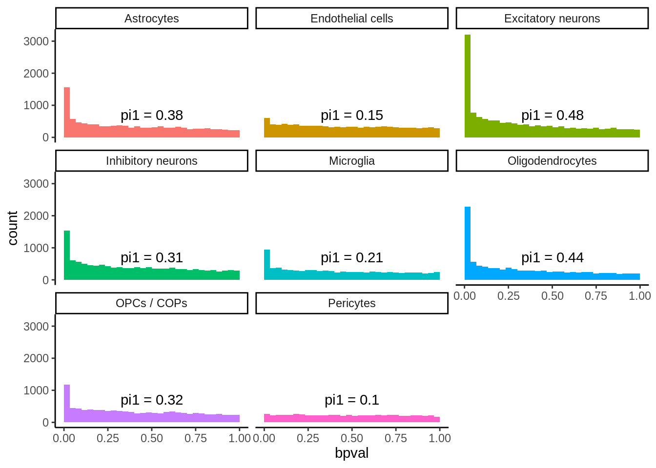
matched_snps <- read_tsv('output/eqtl/eqtl.PC70.metabrain.matched.txt')matched_snps_text <- matched_snps %>%
group_by(cell_type) %>%
summarise(n_rep=sum(p_rep_adj < 0.05),
n_rep_same_direction=sum(p_rep_adj < 0.05 & sign(beta_metabrain)==sign(slope)),
n_tot=n(),
prop_rep=n_rep/n_tot,
prop_rep_same_direction=n_rep_same_direction/n_tot,
prop_rep_same_direction_rep=prop_rep_same_direction/prop_rep,
pi1=ifelse(n()>100,round(1-qvalue::qvalue(p_metabrain)$pi0,digits=2),NA)
) %>%
mutate(p1_label=paste0('Pi1 = ', pi1),
prop_rep_label=paste0('5% FDR = ', round(prop_rep*100,digits=0),'%'),
prop_rep_same_label=paste0('Same direction = ', round(prop_rep_same_direction_rep*100,digits=0),'%'),
label=paste0(prop_rep_label,'\n',prop_rep_same_label,'\n',p1_label)
) %>%
ungroup()`summarise()` ungrouping output (override with `.groups` argument)p <- ggplot(matched_snps,aes(p_metabrain,fill=cell_type)) +
geom_histogram() +
facet_wrap(~cell_type,scales='free_y',nrow=2) +
theme_classic() +
theme(legend.position = 'none') +
geom_text(data=matched_snps_text,aes(x=0.5,y=Inf,vjust=1.1,label=label)) +
ggtitle('Metabrain Cortex matched SNP-gene pairs') +
xlab('Pvalue (Metabrain cortex)')
ggsave(p,filename='output/figures/FigureS3A.png',width=12,height=3,dpi=300)
p
Past versions of unnamed-chunk-92-1.png
Version
Author
Date
7246d60
Julien Bryois
2022-02-10
non-replicating eQTL
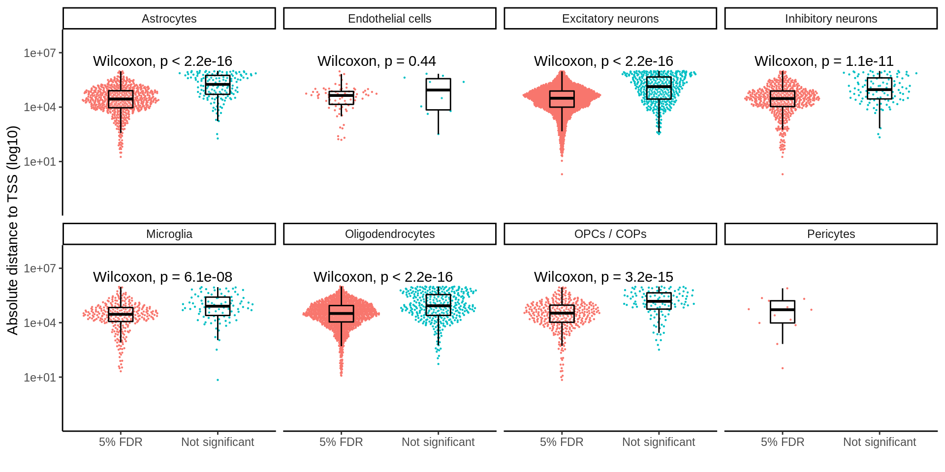
matched_snp_short <- matched_snps %>%
dplyr::select(ensembl,cell_type,SNP,Replication)d <- read_tsv('output/eqtl/eqtl.PC70.txt') %>%
filter(adj_p<0.05) %>%
dplyr::rename(SNP=sid) %>%
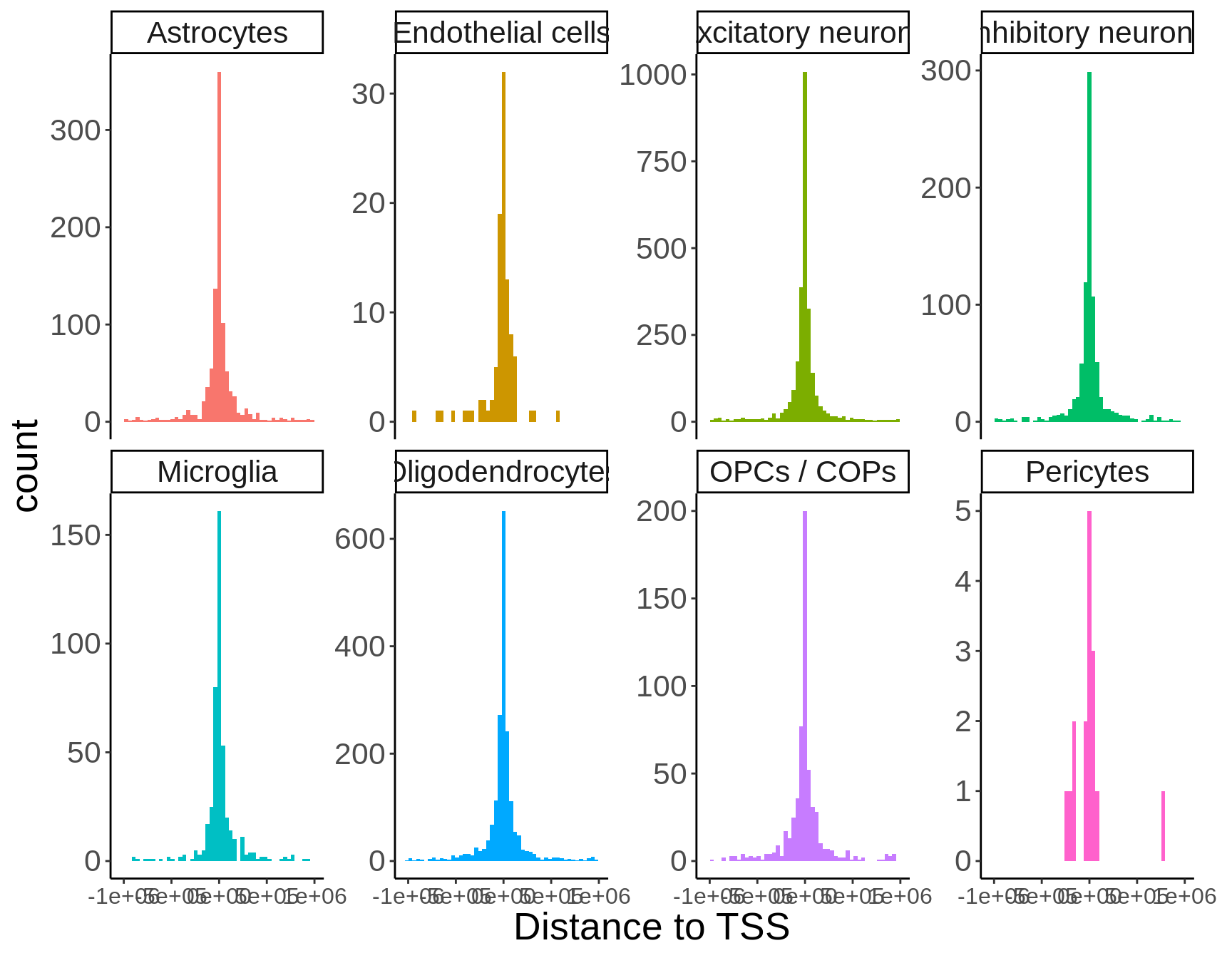
separate(pid,into=c('symbol','ensembl'),sep='_')d_sig <- inner_join(d,matched_snp_short,by=c('ensembl','cell_type','SNP'))p <- ggplot(d_sig,aes(Replication,abs(dist+1),col=Replication)) +
ggbeeswarm::geom_quasirandom(size=0.1) +
geom_boxplot(alpha=0.1,outlier.shape = NA,col='black',width=0.25) +
facet_wrap(~cell_type,nrow=2) +
scale_y_log10(expand=c(0.4,0)) +
ggpubr::stat_compare_means(vjust = -0.5) +
theme_classic() +
theme(legend.position='none') +
ylab('Absolute distance to TSS (log10)') +
xlab('')
ggsave(p,filename='output/figures/FigureS3C.png',width=12,height=3,dpi=300)
p
Past versions of unnamed-chunk-96-1.png
Version
Author
Date
7246d60
Julien Bryois
2022-02-10
Loeuf
loeuf <- read_tsv('data/gnomad_loeuf/supplementary_dataset_11_full_constraint_metrics.tsv') %>%
  filter(canonical==TRUE) %>%
  dplyr::select(gene,gene_id,transcript,oe_lof_upper,p) %>%
  mutate(oe_lof_upper_bin = ntile(oe_lof_upper, 10)) %>%
  dplyr::rename(ensembl=gene_id) %>%
dplyr::select(-gene,-transcript)d_sig <- inner_join(d_sig,loeuf,by='ensembl')p <- ggplot(d_sig,aes(Replication,oe_lof_upper,col=Replication)) +
ggbeeswarm::geom_quasirandom(size=0.1) +
geom_boxplot(alpha=0.1,outlier.shape = NA,col='black',width=0.25) +
facet_wrap(~cell_type,nrow=2) +
scale_y_continuous(expand=c(0.4,0)) +
ggpubr::stat_compare_means(vjust = -0.5) +
theme_classic() +
theme(legend.position='none') +
ylab("LoF observed/expected upper bound \nfraction (LOEUF)") +
xlab('')
ggsave(p,filename='output/figures/FigureS3B.png',width=12,height=3,dpi=300)
p
Past versions of unnamed-chunk-99-1.png
Version
Author
Date
7246d60
Julien Bryois
2022-02-10
Figure S4 - Effect size discovery vs metabrain
matched_snps <- read_tsv('output/eqtl/eqtl.PC70.metabrain.matched.txt') %>%
mutate(glia_neurons=case_when(
cell_type %in% c('Excitatory neurons','Inhibitory neurons') ~ 'Neurons',
TRUE ~ 'Glia'))Parsed with column specification:
cols(
SNP_id_hg38 = col_character(),
ensembl = col_character(),
AlleleAssessed = col_character(),
beta_metabrain = col_double(),
se_metabrain = col_double(),
p_metabrain = col_double(),
cell_type = col_character(),
symbol = col_character(),
SNP = col_character(),
chr_hg38 = col_double(),
effect_allele = col_character(),
other_allele = col_character(),
slope = col_double(),
se = col_double(),
bpval = col_double(),
adj_p = col_double(),
p_rep_adj = col_double(),
Replication = col_character()
)matched_snps_class <- matched_snps %>% dplyr::mutate(cell_type=glia_neurons)matched_snps <- rbind(matched_snps,matched_snps_class) %>%
dplyr::mutate(cell_type=factor(cell_type,
levels=c('Neurons','Glia','Astrocytes','Endothelial cells','Excitatory neurons','Inhibitory neurons','Microglia','Oligodendrocytes','OPCs / COPs','Pericytes')))null_snps <- read_tsv('output/eqtl/eqtl.PC70.metabrain.matched.null.txt') %>%
mutate(glia_neurons=case_when(
cell_type %in% c('Excitatory neurons','Inhibitory neurons') ~ 'Neurons',
TRUE ~ 'Glia'))Parsed with column specification:
cols(
SNP_id_hg38 = col_character(),
ensembl = col_character(),
AlleleAssessed = col_character(),
beta_metabrain = col_double(),
se_metabrain = col_double(),
p_metabrain = col_double(),
cell_type = col_character(),
symbol = col_character(),
SNP = col_character(),
chr_hg38 = col_double(),
effect_allele = col_character(),
other_allele = col_character(),
slope = col_double(),
se = col_double(),
bpval = col_double(),
adj_p = col_double()
)null_snps_class <- null_snps %>% dplyr::mutate(cell_type=glia_neurons)null_snps <- rbind(null_snps,null_snps_class)cell_types <- unique(matched_snps$cell_type)cor_b <- function(sig,null){
var_e_discovery <- mean(sig$se^2)
var_e_replication <- mean(sig$se_metabrain^2)
re <- cor(null$beta_metabrain,null$slope)
numerator <- cov(sig$beta_metabrain,sig$slope) - re*sqrt(var_e_discovery*var_e_replication)
denominator <- sqrt( (var(sig$slope) - var_e_discovery) * (var(sig$beta_metabrain) - var_e_replication) )
out <- numerator/denominator
return(out)
}rb_res <- lapply(cell_types,function(cell_type_name){
sig_cell <- filter(matched_snps,cell_type==cell_type_name)
null_snps_cell <- filter(null_snps,cell_type==cell_type_name)
rb <- cor_b(sig_cell,null_snps_cell)
pearson <- cor(sig_cell$beta_metabrain,sig_cell$slope)
spearman <- cor(sig_cell$beta_metabrain,sig_cell$slope,method='spearman')
out <- tibble(cell_type=cell_type_name,rb=rb,cor_pearson=pearson,cor_spearman=spearman)
return(out)
}) %>%
bind_rows() %>%
arrange(rb)matched_snps_text <- matched_snps %>%
group_by(cell_type) %>%
summarise(n_rep=sum(p_rep_adj < 0.05),
n_rep_same_direction=sum(p_rep_adj < 0.05 & sign(beta_metabrain)==sign(slope)),
n_tot=n(),
prop_rep=n_rep/n_tot,
prop_rep_same_direction=n_rep_same_direction/n_tot,
prop_rep_same_direction_rep=prop_rep_same_direction/prop_rep,
pi1=ifelse(n()>100,round(1-qvalue::qvalue(p_metabrain)$pi0,digits=2),NA)
) %>%
inner_join(.,rb_res,by='cell_type') %>%
mutate(p1_label=paste0('Pi1 = ', pi1),
prop_rep_label=paste0('5% FDR = ', round(prop_rep*100,digits=0),'%'),
prop_rep_same_label=paste0('Same direction = ', round(prop_rep_same_direction_rep*100,digits=0),'%'),
rb_label=paste0('Rb = ',round(rb,digits=2)),
label=paste0(prop_rep_label,'\n',prop_rep_same_label,'\n',p1_label,'\n',rb_label)
) %>%
ungroup() %>%
dplyr::mutate(cell_type=factor(cell_type,
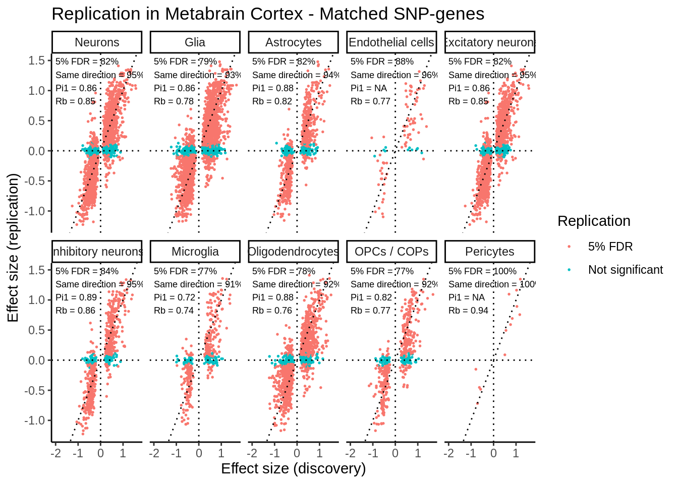
levels=c('Neurons','Glia','Astrocytes','Endothelial cells','Excitatory neurons','Inhibitory neurons','Microglia','Oligodendrocytes','OPCs / COPs','Pericytes')))`summarise()` ungrouping output (override with `.groups` argument)p <- ggplot(matched_snps,aes(slope,beta_metabrain,col=Replication)) +
geom_point(size=0.3) +
facet_wrap(~cell_type,nrow=2) +
theme_classic() +
geom_hline(yintercept = 0,linetype=3) +
geom_vline(xintercept = 0,linetype=3) +
geom_abline(linetype=3) +
xlab('Effect size (discovery)') +
ylab('Effect size (replication)') +
geom_text(data=matched_snps_text,aes(x=-2,y=Inf,vjust=1.1,hjust = 0,label=label),size=2.4,inherit.aes = FALSE) +
ggtitle('Replication in Metabrain Cortex - Matched SNP-genes')
ggsave(p,filename='output/figures/FigureS4.png',width=13,dpi=300,height=5)
p
Past versions of unnamed-chunk-110-1.png
Version
Author
Date
865a38a
Julien Bryois
2022-02-10
Figure S5 - Cell type vs tissue-like
d <- read_tsv('output/eqtl/eqtl.PC70.txt') %>%
dplyr::count(adj_p<0.05) %>%
filter(`adj_p < 0.05`)
d_pb <- read_tsv('output/eqtl/eqtl.pb.PC70.txt') %>%
dplyr::count(adj_p<0.05)%>%
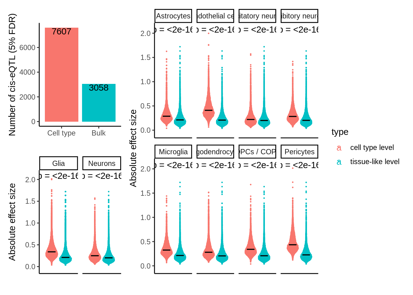
filter(`adj_p < 0.05`)p1 <- tibble(`Cell type`=d$n,Bulk=d_pb$n) %>%
gather(type,value) %>%
mutate(type=factor(type,levels=c('Cell type','Bulk'))) %>%
ggplot(.,aes(type,value,fill=type)) +
geom_col() +
theme_classic() +
xlab('') +
ylab('Number of cis-eQTL (5% FDR)') +
theme(legend.position = 'none') +
geom_text(aes(label=value,vjust=1.1))cell_type <- read_tsv('output/eqtl/eqtl.PC70.txt') %>%
dplyr::select(cell_type=cell_type,pid,slope_cell=slope)Parsed with column specification:
cols(
cell_type = col_character(),
pid = col_character(),
nvar = col_double(),
shape1 = col_double(),
shape2 = col_double(),
dummy = col_double(),
sid = col_character(),
dist = col_double(),
npval = col_double(),
slope = col_double(),
ppval = col_double(),
bpval = col_double(),
adj_p = col_double()
)bulk <- read_tsv('output/eqtl/eqtl.pb.PC70.txt') %>%
dplyr::select(tissue=cell_type,pid,slope_tissue=slope)Parsed with column specification:
cols(
cell_type = col_character(),
pid = col_character(),
nvar = col_double(),
shape1 = col_double(),
shape2 = col_double(),
dummy = col_double(),
sid = col_character(),
dist = col_double(),
npval = col_double(),
slope = col_double(),
ppval = col_double(),
bpval = col_double(),
adj_p = col_double()
)d <- inner_join(cell_type,bulk,by='pid')p2 <- d %>% gather(type,value,-cell_type,-tissue,-pid) %>%
mutate(type=ifelse(type=='slope_cell','cell type level','tissue-like level')) %>%
filter(value<6*sd(value)) %>% #filter out outliers (effect sizes >6sd from the mean)
mutate(cell_type=ifelse(grepl('neurons',cell_type),'Neurons','Glia')) %>%
ggplot(.,aes(cell_type,abs(value),col=type)) +
ggbeeswarm::geom_quasirandom(dodge.width = 0.9,size=0.2) +
ggpubr::stat_compare_means(aes(group = type),label = "p.format") +
stat_summary(fun = median,
fun.min = median,
fun.max = median,
geom = "crossbar",
width = 0.5,
size=0.25,
color='black',
position = position_dodge(width = 0.9),
aes(group=type)
) +
xlab('') +
ylab('Absolute effect size') +
theme_classic() +
facet_wrap(~cell_type,ncol=4,scales = 'free_x') +
theme(axis.text.x = element_blank(), axis.ticks.x = element_blank(),legend.position = 'none') +
scale_y_continuous(expand=c(0.1,0))p3 <- d %>% gather(type,value,-cell_type,-tissue,-pid) %>%
mutate(type=ifelse(type=='slope_cell','cell type level','tissue-like level')) %>%
filter(value<6*sd(value)) %>% #filter out outliers (effect sizes >6sd from the mean)
ggplot(.,aes(cell_type,abs(value),col=type))+
ggbeeswarm::geom_quasirandom(dodge.width = 0.9,size=0.2) +
ggpubr::stat_compare_means(aes(group = type),label = "p.format") +
stat_summary(fun = median,
fun.min = median,
fun.max = median,
geom = "crossbar",
width = 0.5,
size=0.25,
color='black',
position = position_dodge(width = 0.9),
aes(group=type)
) +
xlab('') +
ylab('Absolute effect size') +
theme_classic() +
facet_wrap(~cell_type,ncol=4,scales = 'free_x') +
theme(axis.text.x = element_blank(), axis.ticks.x = element_blank()) +
scale_y_continuous(expand=c(0.1,0))p <-((p1 / p2 + plot_layout(guides = 'auto')) | p3) + plot_layout(guides = 'collect',widths = c(1, 2))
ggsave(p,filename='output/figures/FigureS5.png',width=10,dpi=300,height=6)
p
Past versions of unnamed-chunk-117-1.png
Version
Author
Date
865a38a
Julien Bryois
2022-02-10
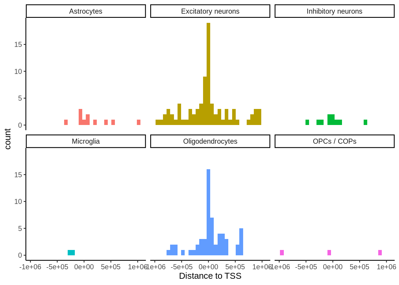
Figure S6/S7 eQTL location
snp_positions_file <- 'data_sensitive/genotypes/processed/snp_pos_hg38.txt'
snp_coordinates <- data.table::fread(snp_positions_file,header = FALSE,data.table = FALSE) %>%
setNames(c('chr','start','sid')) %>%
as_tibble()dir.create('data_sensitive/eqtl/PC70/location',showWarnings = FALSE)
d <- read_tsv('output/eqtl/eqtl.PC70.txt') %>%
filter(adj_p<0.05) %>%
dplyr::select(cell_type,pid,sid) %>%
unique() %>%
left_join(.,snp_coordinates,by='sid') %>%
mutate(start=as.numeric(start),
end=start) %>%
dplyr::select(chr,start,end,sid,pid,cell_type) %>%
mutate(chr=paste0('chr',chr)) %>%
arrange(chr,start,end) %>%
write_tsv(.,'data_sensitive/eqtl/PC70/location/eqtl_5FDR.bed',col_names = FALSE)gtf <- rtracklayer::import('data/gencode/Homo_sapiens.GRCh38.96.filtered.gtf') %>%
as.data.frame() %>%
filter(type=='gene') %>%
mutate(gene_label=gsub('\\..+','',gene_id)) %>%
mutate(score='.') %>%
dplyr::select(seqnames,start,end,gene_label,score,strand) %>%
filter(seqnames %in% paste0(1:22)) %>%
mutate(seqnames=as.character(paste0('chr',seqnames))) %>%
arrange(seqnames,start,end) %>%
write_tsv('data_sensitive/eqtl/PC70/location/Homo_sapiens.GRCh38.96.filtered.1_22.bed',col_names = FALSE)cd data_sensitive/eqtl/PC70/location/
ml bedtools/2.25.0-goolf-1.7.20
bedtools closest -D b -k 500 -a eqtl_5FDR.bed -b Homo_sapiens.GRCh38.96.filtered.1_22.bed > eqtl_5FDR.closest_gene.bedclosest <- data.table::fread('data_sensitive/eqtl/PC70/location/eqtl_5FDR.closest_gene.bed',header = FALSE,data.table = FALSE) %>%
dplyr::select(-V7,-V8,-V9,-V11,-V12) %>%
setNames(c(colnames(d),'closest_gene','distance')) %>%
group_by(sid,pid,cell_type) %>%
mutate(rank=rank(abs(distance),ties.method='min')) %>%
ungroup() %>%
separate(pid,into=c('symbol','ensembl'),sep='_',remove = FALSE)
Gene body location
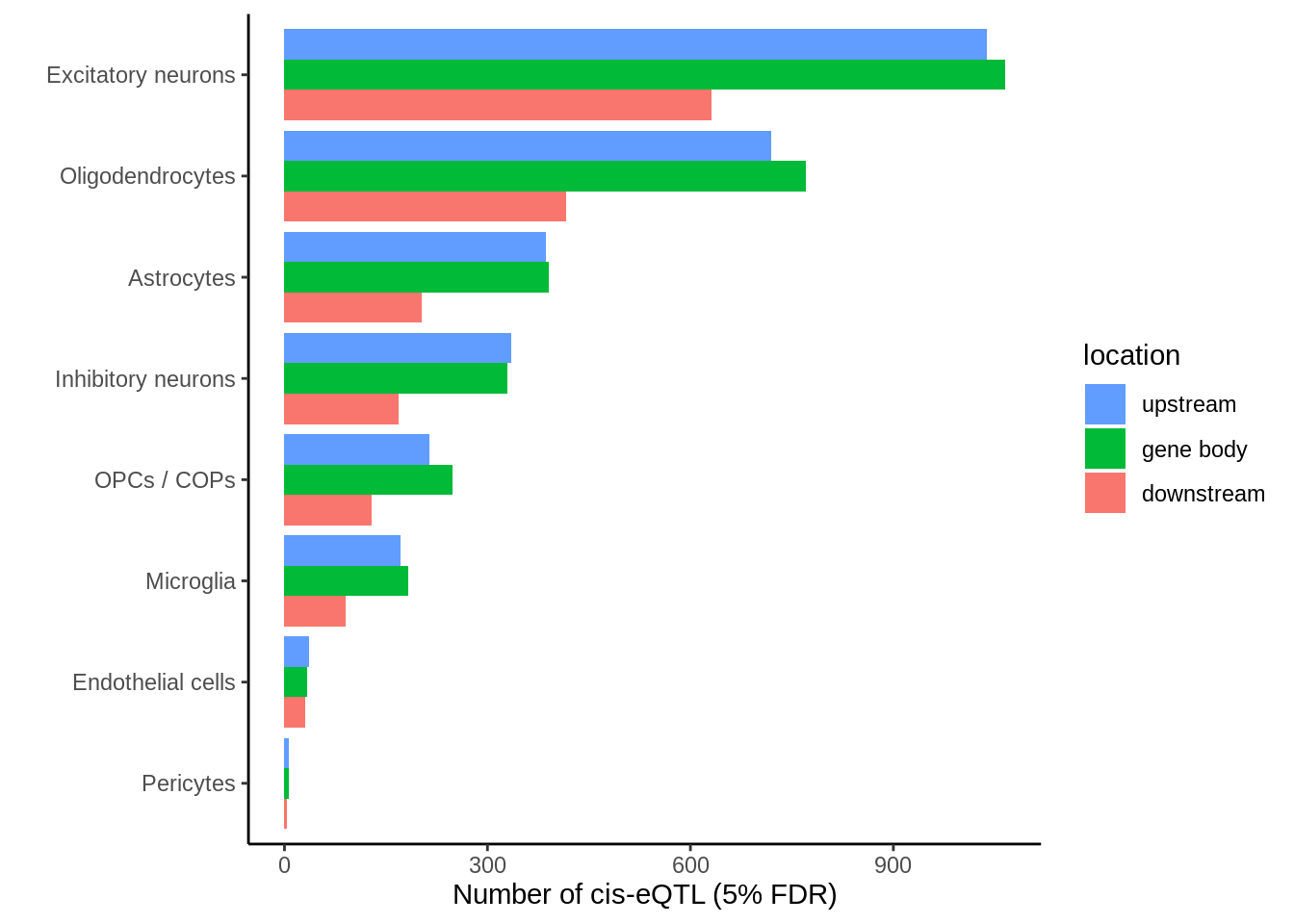
p <- closest %>%
filter(ensembl==closest_gene) %>%
mutate(location=case_when(
distance < 0 ~ 'upstream',
distance == 0 ~ 'gene body',
distance > 0 ~ 'downstream')) %>%
dplyr::count(cell_type,location) %>%
group_by(cell_type) %>%
mutate(tot=sum(n),prop=round(n*100/tot,digits=2)) %>%
ggplot(.,aes(reorder(cell_type,n),n,fill=location)) +
geom_col(position=position_dodge()) +
coord_flip() +
guides(fill = guide_legend(reverse=T)) +
theme_classic() +
ylab('Number of cis-eQTL (5% FDR)') +
xlab('')
ggsave(p,filename='output/figures/FigureS6.png',width=5,height=3,dpi=300)
p
Past versions of unnamed-chunk-123-1.png
Version
Author
Date
865a38a
Julien Bryois
2022-02-10
7246d60
Julien Bryois
2022-02-10
f999a54
Julien Bryois
2022-02-02
bb7b4d3
Julien Bryois
2022-01-28
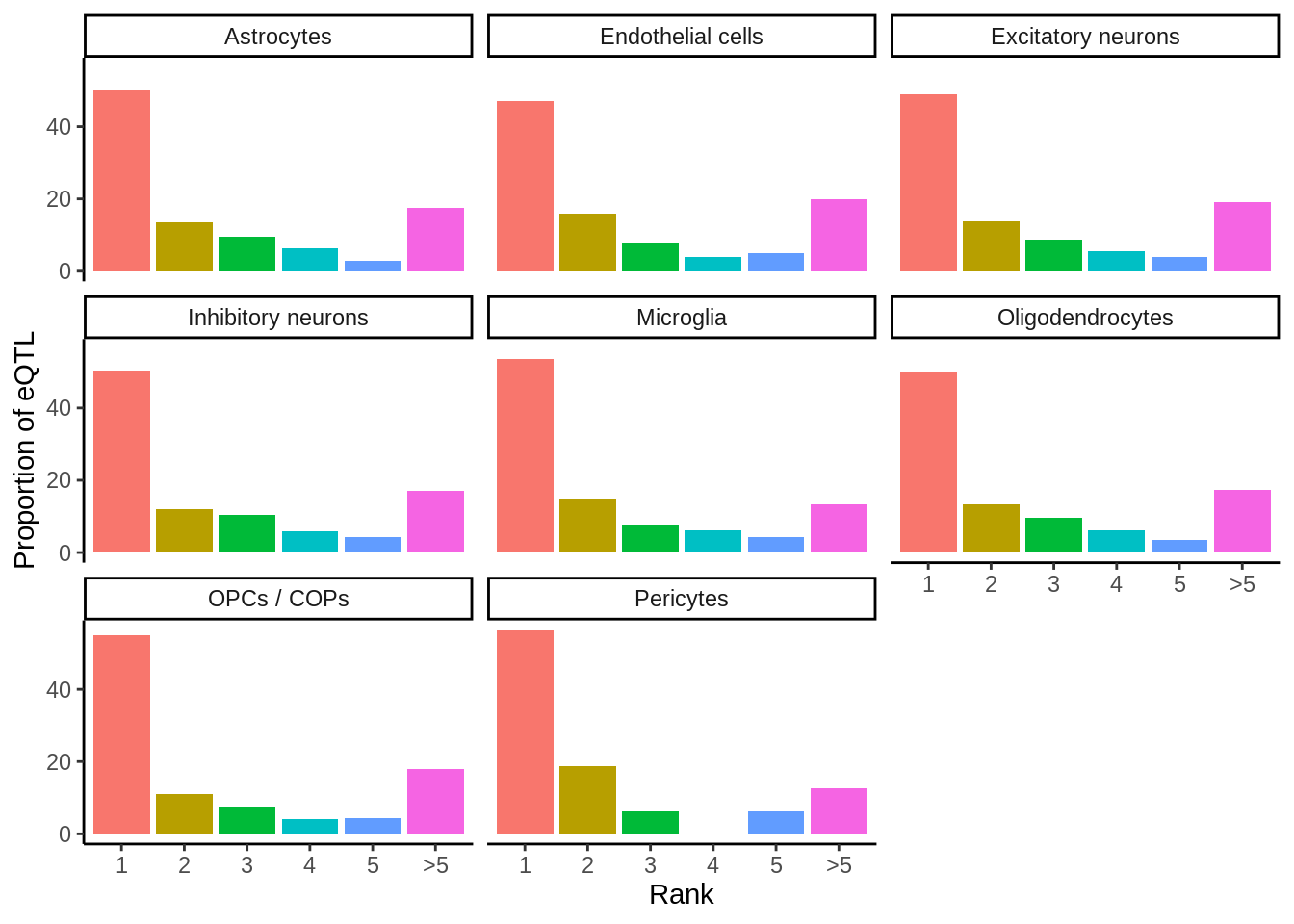
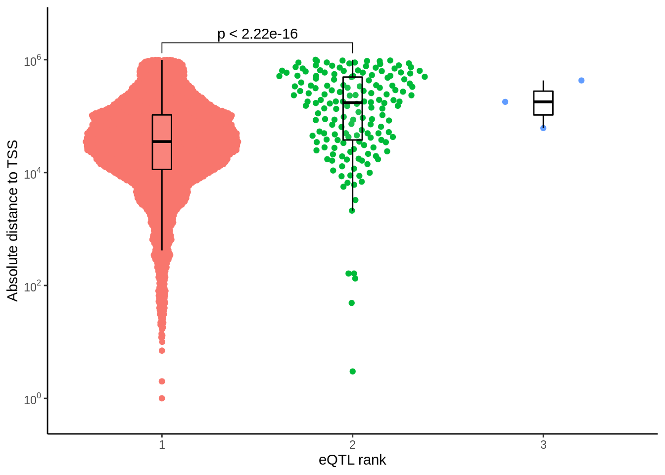
Rank of affected gene
prop_closest <- closest %>% filter(ensembl==closest_gene) %>%
mutate(rank=ifelse(rank>5,'>5',rank)) %>%
dplyr::count(cell_type,rank) %>%
add_count(cell_type) %>%
mutate(prop=round(n*100/nn,digits=2)) %>%
mutate(rank=factor(rank,levels=c('1','2','3','4','5','>5'))) %>%
arrange(cell_type,rank)p <- ggplot(prop_closest,aes(rank,prop,fill=rank)) +
geom_col() +
facet_wrap(~cell_type) +
theme_classic() +
theme(legend.position = 'none') +
xlab('Rank') +
ylab('Proportion of eQTL')
ggsave(p,filename='output/figures/FigureS7.png',width=6,dpi=300)
p
Past versions of unnamed-chunk-125-1.png
Version
Author
Date
865a38a
Julien Bryois
2022-02-10
Figure S8 - eQTL expression level
d <- read_tsv('output/eqtl/eqtl.PC70.txt')exp_files <- list.files('data_sensitive/eqtl/',pattern = '.bed.gz$',full.names = T)read_exp_get_median <- function(i){
cell_type <- basename(exp_files[i]) %>%
gsub('\\.bed.gz','',.) %>%
gsub('\\.',' ',.) %>%
gsub('OPCs COPs','OPCs / COPs',.)
exp_df <- read_tsv(exp_files[i]) %>% dplyr::select(-`#Chr`,-start,-end) %>% column_to_rownames('ID') %>% as.matrix()
medians_per_gene <- matrixStats::rowMedians(exp_df) %>%
setNames(rownames(exp_df)) %>%
as.data.frame() %>%
setNames('median_cpm') %>%
rownames_to_column('pid') %>%
mutate(cell_type=cell_type)
return(medians_per_gene)
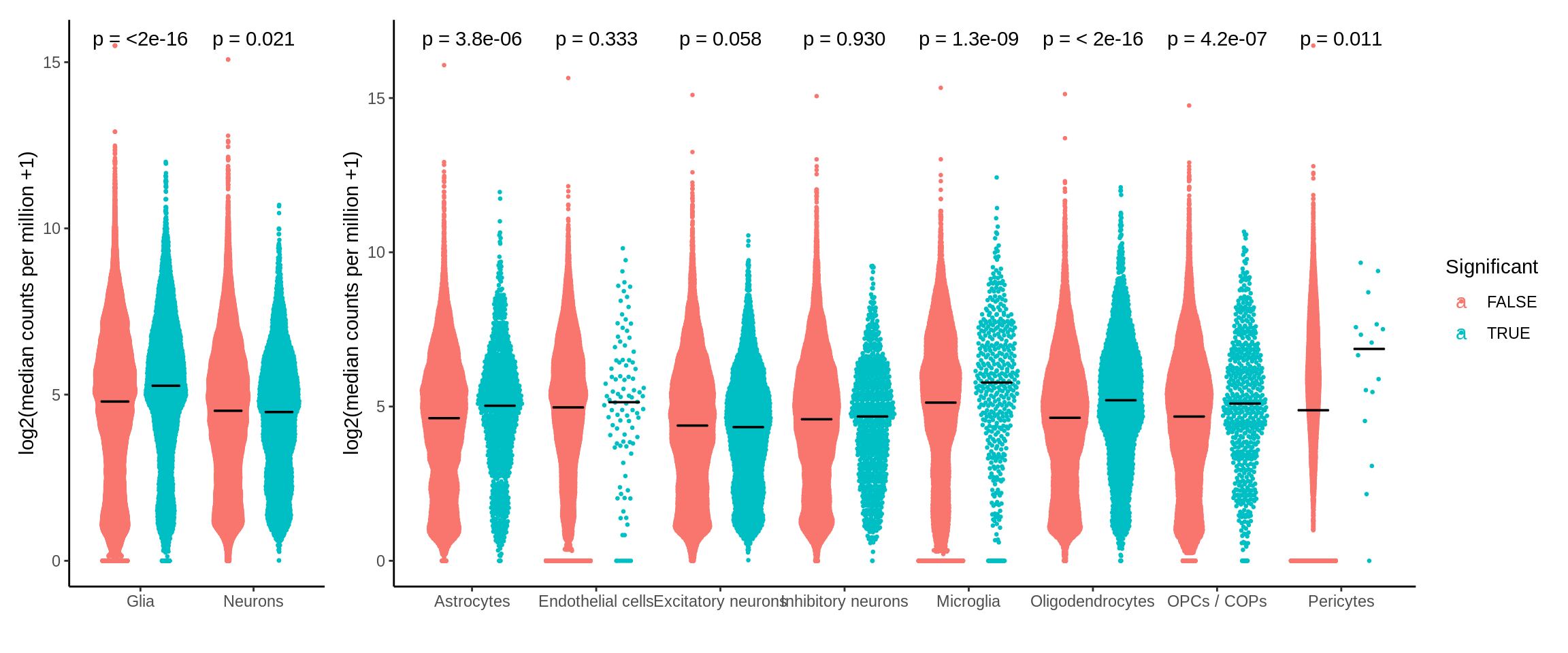
}median_expression_all <- mclapply(1:length(exp_files),function(i) read_exp_get_median(i),mc.cores = 8) %>% bind_rows()d_cpm <- left_join(d,median_expression_all,by=c('cell_type','pid')) %>% mutate(Significant=ifelse(adj_p<0.05,TRUE,FALSE))p2 <- ggplot(d_cpm,aes(cell_type,log2(median_cpm+1),col=Significant)) +
theme_classic() +
ggbeeswarm::geom_quasirandom(dodge.width = 0.9,size=0.5) +
ggpubr::stat_compare_means(aes(group = Significant),label = "p.format") +
ylab('log2(median counts per million +1)') +
xlab('') +
stat_summary(fun = median,
fun.min = median,
fun.max = median,
geom = "crossbar",
width = 0.5,
size=0.25,
color='black',
position = position_dodge(width = 0.9),
aes(group=Significant)
)d_cpm <- d_cpm %>% mutate(type=ifelse(grepl('neurons',cell_type),'Neurons','Glia')) %>%
group_by(type,pid) %>%
mutate(median_cpm2=median(median_cpm))p1 <- ggplot(d_cpm,aes(type,log2(median_cpm2+1),col=Significant)) +
theme_classic() +
ggbeeswarm::geom_quasirandom(size=0.5,dodge.width = 0.9) +
ggpubr::stat_compare_means(aes(group = Significant),label = "p.format") +
ylab('log2(median counts per million +1)') +
xlab('') +
stat_summary(fun = median,
fun.min = median,
fun.max = median,
geom = "crossbar",
width = 0.5,
size=0.25,
color='black',
position = position_dodge(width = 0.9),
aes(group=Significant)) +
theme(legend.position='none')p <- p1 + p2 + plot_layout(widths = c(1, 4))
ggsave(p,filename='output/figures/FigureS8.png',width=14,height=5,dpi=300)
p
Past versions of unnamed-chunk-134-1.png
Version
Author
Date
865a38a
Julien Bryois
2022-02-10
7246d60
Julien Bryois
2022-02-10
f999a54
Julien Bryois
2022-02-02
bb7b4d3
Julien Bryois
2022-01-28
Figure S9 LOEUF eQTL
loeuf <- read_tsv('data/gnomad_loeuf/supplementary_dataset_11_full_constraint_metrics.tsv') %>%
  filter(canonical==TRUE) %>%
  dplyr::select(gene,gene_id,transcript,oe_lof_upper,p) %>%
  mutate(oe_lof_upper_bin = ntile(oe_lof_upper, 10)) %>%
  dplyr::rename(ensembl=gene_id) %>%
dplyr::select(-gene,-transcript)Parsed with column specification:
cols(
.default = col_double(),
gene = col_character(),
transcript = col_character(),
canonical = col_logical(),
constraint_flag = col_character(),
transcript_type = col_character(),
gene_id = col_character(),
gene_type = col_character(),
brain_expression = col_logical(),
chromosome = col_character()
)See spec(...) for full column specifications.d_loeuf <- read_tsv('output/eqtl/eqtl.PC70.txt') %>%
separate(pid,into=c('symbol','ensembl'),sep='_') %>%
left_join(.,loeuf,by='ensembl') %>%
mutate(Significant=ifelse(adj_p<0.05,TRUE,FALSE)) %>%
filter(!is.na(oe_lof_upper))Parsed with column specification:
cols(
cell_type = col_character(),
pid = col_character(),
nvar = col_double(),
shape1 = col_double(),
shape2 = col_double(),
dummy = col_double(),
sid = col_character(),
dist = col_double(),
npval = col_double(),
slope = col_double(),
ppval = col_double(),
bpval = col_double(),
adj_p = col_double()
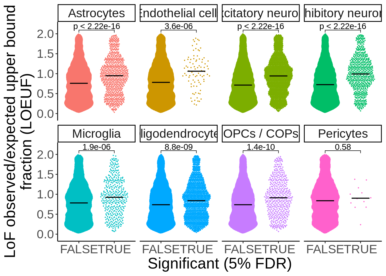
)my_comparisons <- list( c("FALSE","TRUE"))
p <- ggplot(d_loeuf,aes(Significant,oe_lof_upper,col=cell_type)) + ggbeeswarm::geom_quasirandom(size=0.1) + facet_wrap(~cell_type,ncol=4,nrow=2) + theme_classic() + theme(legend.position='none',text=element_text(size=20)) + stat_summary(fun = median, fun.min = median, fun.max = median,
geom = "crossbar", width = 0.5,size=0.25,color='black') + xlab("Significant (5% FDR)") + ylab("LoF observed/expected upper bound
fraction (LOEUF)") + ggpubr::stat_compare_means(comparisons = my_comparisons) + scale_y_continuous(expand=c(0.1,0))
ggsave(p,filename='output/figures/FigureS9A.png',height=7,width=11,dpi = 300)
p
Past versions of unnamed-chunk-137-1.png
Version
Author
Date
865a38a
Julien Bryois
2022-02-10
LOEUF eQTL vs bulk
#eQTL bulk (aggregate across all cells from and invididual)
d_pb <- read_tsv('output/eqtl/eqtl.pb.PC70.txt') %>%
dplyr::select(pid,adj_p_pb=adj_p) %>%
separate(pid,into=c('symbol','ensembl'),sep='_')loeuf <- read_tsv('data/gnomad_loeuf/supplementary_dataset_11_full_constraint_metrics.tsv') %>%
filter(canonical==TRUE) %>%
dplyr::select(gene,gene_id,transcript,oe_lof_upper,p) %>%
mutate(oe_lof_upper_bin = ntile(oe_lof_upper, 10)) %>%
dplyr::rename(ensembl=gene_id) %>%
dplyr::select(-gene,-transcript)d_loeuf <- read_tsv('output/eqtl/eqtl.PC70.txt') %>%
separate(pid,into=c('symbol','ensembl'),sep='_') %>%
left_join(.,loeuf,by='ensembl') %>%
filter(!is.na(oe_lof_upper)) %>%
inner_join(.,d_pb,by=c('ensembl','symbol')) %>%
mutate(Significant=factor(case_when(
adj_p<0.05 & adj_p_pb <0.05 ~ "Both",
adj_p<0.05 & adj_p_pb >=0.05 ~ "Cell",
adj_p>=0.05 & adj_p_pb <0.05 ~ "Bulk",
adj_p>=0.05 & adj_p_pb >=0.05 ~ "None"),
levels=c('None','Cell','Bulk','Both')))Parsed with column specification:
cols(
cell_type = col_character(),
pid = col_character(),
nvar = col_double(),
shape1 = col_double(),
shape2 = col_double(),
dummy = col_double(),
sid = col_character(),
dist = col_double(),
npval = col_double(),
slope = col_double(),
ppval = col_double(),
bpval = col_double(),
adj_p = col_double()
)agg_all <- d_loeuf %>%
dplyr::select(ensembl,oe_lof_upper,adj_p,adj_p_pb) %>%
group_by(ensembl,oe_lof_upper) %>%
summarise(sig_cell_type=ifelse(sum(adj_p<0.05)>0,TRUE,FALSE),
sig_bulk=ifelse(sum(adj_p_pb<0.05)>0,TRUE,FALSE)) %>%
mutate(Significant=factor(case_when(
sig_cell_type==TRUE & sig_bulk==TRUE ~ "Both",
sig_cell_type==TRUE & sig_bulk==FALSE ~ "Cell",
sig_cell_type==FALSE & sig_bulk==TRUE ~ "Bulk",
sig_cell_type==FALSE & sig_bulk==FALSE ~ "None"),
levels=c('None','Cell','Bulk','Both'))) %>%
mutate(cell_type='All') %>%
ungroup() %>%
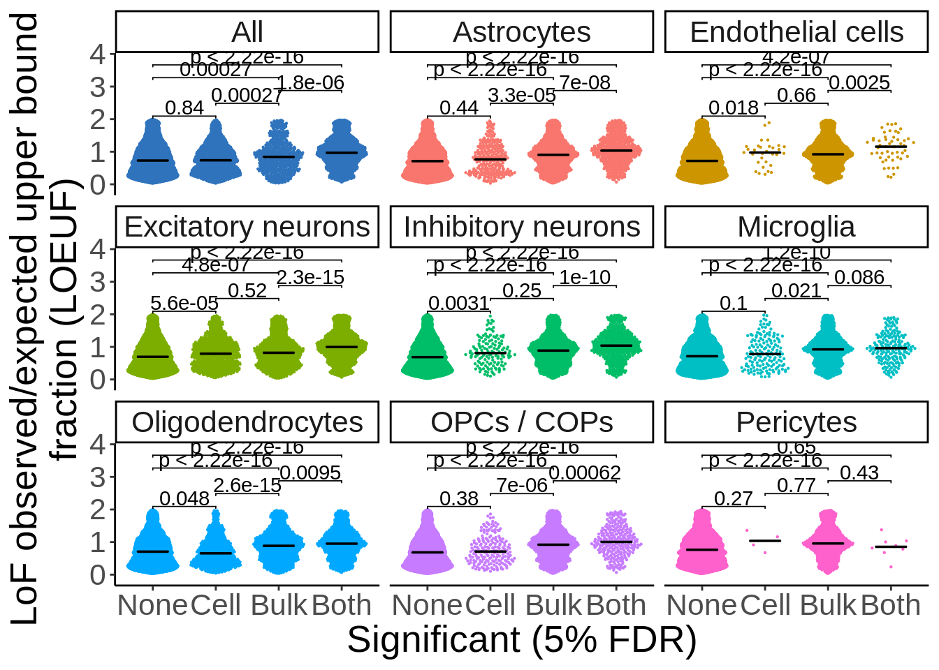
dplyr::select(cell_type,oe_lof_upper,Significant)`summarise()` regrouping output by 'ensembl' (override with `.groups` argument)d_loeuf_short <- d_loeuf %>% dplyr::select(cell_type,oe_lof_upper,Significant)all <- rbind(agg_all,d_loeuf_short)my_comparisons <- list( c("None","Cell"),
c("Cell","Bulk"),
c("Bulk","Both"),
c("None","Bulk"),
c("None","Both")
)p <- all %>% ggplot(.,aes(Significant,oe_lof_upper,col=cell_type)) + ggbeeswarm::geom_quasirandom(size=0.1) + facet_wrap(~cell_type,nrow=3) + theme_classic() + theme(legend.position='none',text=element_text(size=20)) + stat_summary(fun = median, fun.min = median, fun.max = median,
geom = "crossbar", width = 0.5,size=0.25,color='black') + xlab("Significant (5% FDR)") + ylab("LoF observed/expected upper bound
fraction (LOEUF)") + ggpubr::stat_compare_means(comparisons = my_comparisons,step.increase = 0.2) + scale_y_continuous(expand=c(0.1,0)) +
scale_color_manual(values=c('#2e73bc',hue_pal()(8)))
ggsave(p,filename='output/figures/FigureS9B.png',width = 11,height=7,dpi = 300)
p
Past versions of unnamed-chunk-145-1.png
Version
Author
Date
865a38a
Julien Bryois
2022-02-10
7246d60
Julien Bryois
2022-02-10
Figure S11 - CaVEMan
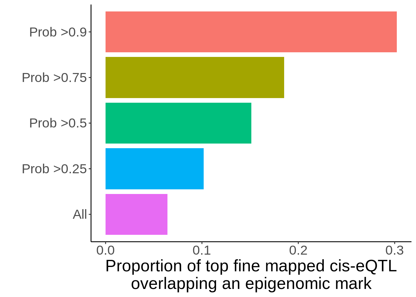
Epigenome overlap
d <- read_tsv('output/eqtl/eqtl.70PCs.caveman.txt')path <- system.file(package="liftOver", "extdata", "hg38ToHg19.over.chain")
ch <- import.chain(path)dir.create('data_sensitive/eqtl/PC70_caveman/epigenome_overlap',showWarnings = FALSE)
bed_hg19 <- d %>% separate(GENE,into=c('symbol','ensembl','chr','start','A1','A2'),sep='_') %>%
mutate(chr=paste0('chr',chr)) %>%
mutate(end=start) %>%
dplyr::select(chr,start,end,cell_type,symbol,ensembl,Probability) %>%
GenomicRanges::makeGRangesFromDataFrame(., TRUE) %>%
liftOver(.,ch) %>%
unlist() %>%
as.data.frame() %>%
as_tibble() %>%
arrange(seqnames,start) %>%
unique() %>%
write_tsv(.,'data_sensitive/eqtl/PC70_caveman/epigenome_overlap/finemapped_SNPs.bed',col_names = FALSE)cd data_sensitive/eqtl/PC70_caveman/epigenome_overlap/
source ~/.bashrc
ml bedtools/2.25.0-goolf-1.7.20
ln -s ../../../../data/gwas_epigenome_overlap/corces_hg19.bed .
bedtools intersect -loj -wa -wb -a finemapped_SNPs.bed -b corces_hg19.bed > finemapped_epigenomic_marks.bedd <- read_tsv('data_sensitive/eqtl/PC70_caveman/epigenome_overlap/finemapped_epigenomic_marks.bed',col_names = FALSE) %>% setNames(c(colnames(bed_hg19),'chr_epi','start_epi','end_epi','study','cell_type_epi','specific','Annotation')) %>%
mutate(id=paste(seqnames,start,end,cell_type,symbol,sep='_')) %>%
dplyr::select(-width,-strand) %>%
mutate(has_overlap=ifelse(chr_epi!='.','Overlap','No overlap'))p <- d %>%
mutate(any_overlap=ifelse(chr_epi=='.','no_overlap','overlap')) %>%
dplyr::select(id,any_overlap,Probability) %>% unique() %>%
group_by(any_overlap) %>%
summarise(`All`=n(),
`Prob >0.25`=sum(Probability>0.25),
`Prob >0.5`=sum(Probability>0.5),
`Prob >0.75`=sum(Probability>0.75),
`Prob >0.9`=sum(Probability>0.9)) %>%
gather(filter,value,-any_overlap) %>%
group_by(filter) %>%
mutate(tot=sum(value)) %>%
mutate(prop=value/tot) %>%
filter(any_overlap=='overlap') %>%
ggplot(.,aes(filter,prop,fill=filter))+geom_col(position = position_dodge()) + xlab('') + ylab('Proportion of top fine mapped cis-eQTL\noverlapping an epigenomic mark') + theme_classic() + guides(fill=guide_legend(reverse = TRUE)) + scale_fill_hue(direction=-1) + theme(legend.position='none',text=element_text(size=20)) + coord_flip()
ggsave(p,filename=paste0('output/figures/FigureS11A.png'),width=7,height=4,dpi=300)
p
Past versions of unnamed-chunk-155-1.png
Version
Author
Date
865a38a
Julien Bryois
2022-02-10
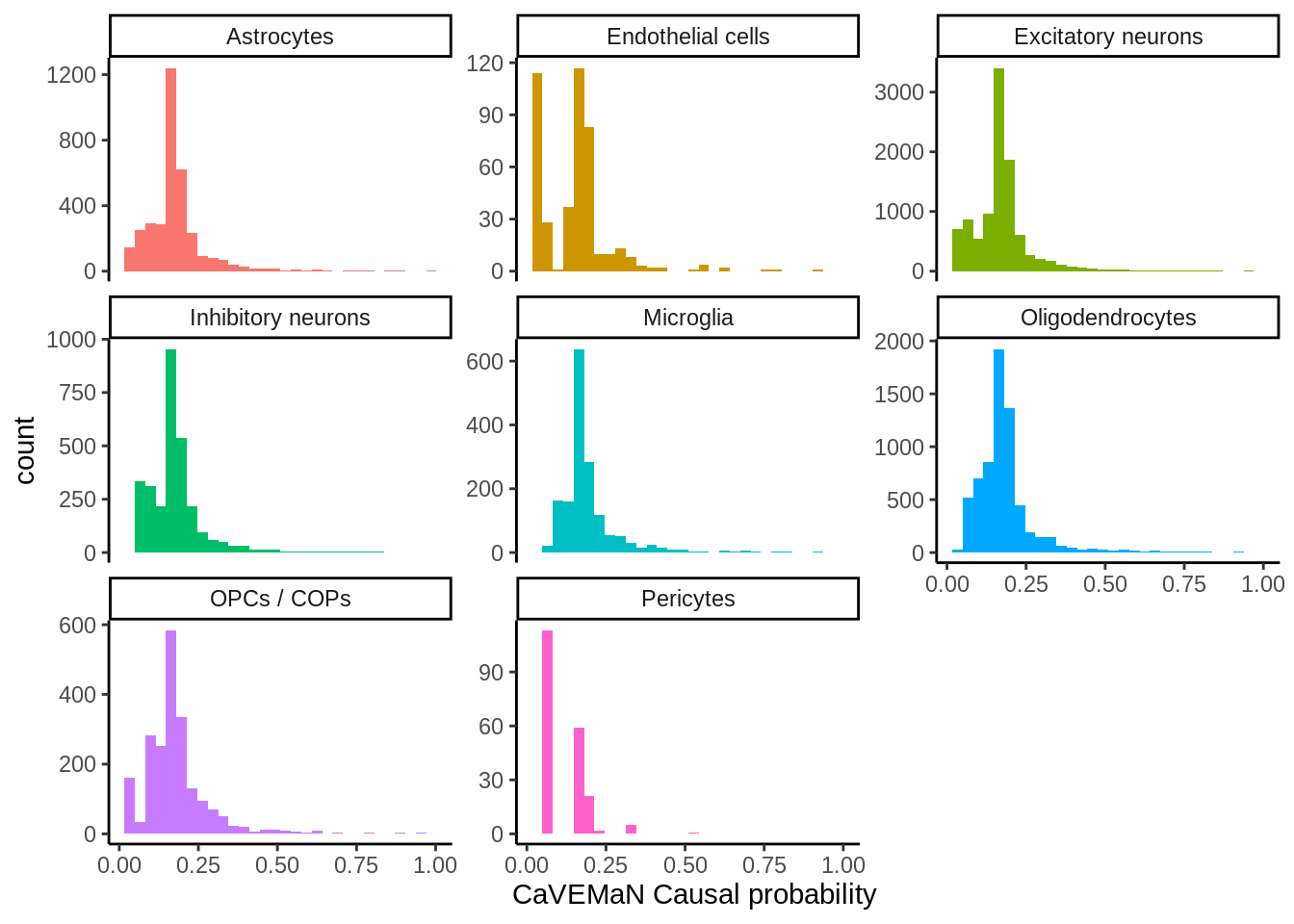
Histogram
d <- read_tsv('output/eqtl/eqtl.70PCs.caveman.txt')p <- ggplot(d,aes(Probability,fill=cell_type)) +
geom_histogram() +
theme_classic() +
xlab('CaVEMaN Causal probability') +
theme(legend.position='none') +
facet_wrap(~cell_type,scales='free_y')
ggsave(p,filename='output/figures/FigureS11B.png',width=5,height=3,dpi=300)
p
Past versions of unnamed-chunk-157-1.png
Version
Author
Date
865a38a
Julien Bryois
2022-02-10
7246d60
Julien Bryois
2022-02-10
f999a54
Julien Bryois
2022-02-02
bb7b4d3
Julien Bryois
2022-01-28
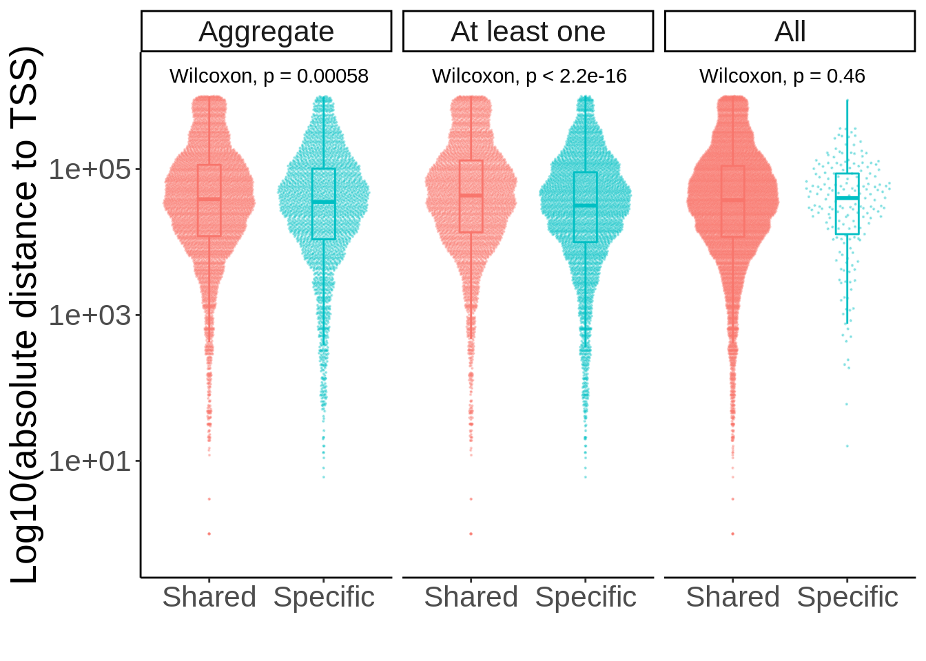
Figure S15 - cell type specific eQTL
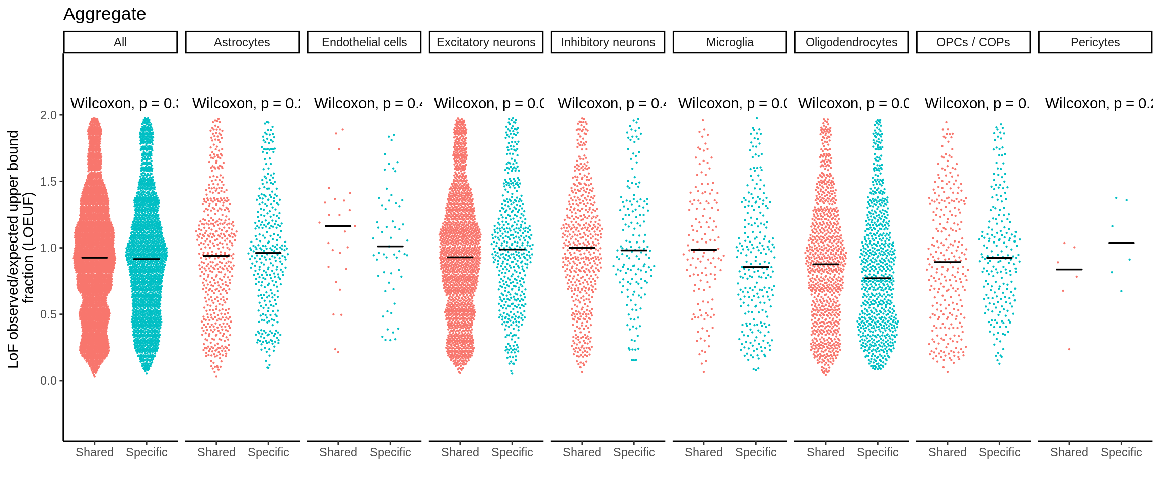
PLOEUF
loeuf <- read_tsv('data/gnomad_loeuf/supplementary_dataset_11_full_constraint_metrics.tsv') %>%
  filter(canonical==TRUE) %>%
  dplyr::select(gene,gene_id,transcript,oe_lof_upper,p) %>%
  mutate(oe_lof_upper_bin = ntile(oe_lof_upper, 10)) %>%
  dplyr::rename(ensembl=gene_id) %>%
dplyr::select(-gene,-transcript)d <- read_tsv('output/eqtl_specific/eqtl.PC70.specific.txt') %>%
#Sets pvalue to NA if the model did not converge
mutate(nb_pvalue_aggregate=ifelse(nb_pvalue_aggregate_model_converged==FALSE,NA,nb_pvalue_aggregate)) %>%
mutate(nb_pvalue_at_least_one=ifelse(nb_pvalue_at_least_one_model_converged==FALSE,NA,nb_pvalue_at_least_one)) %>% #Remove genes for which the model did not converge (9 genes)
filter(!is.na(nb_pvalue_aggregate),
!is.na(nb_pvalue_at_least_one),
nb_pvalue_at_least_one!=Inf) %>%
#Get adjusted pvalues
mutate(nb_pvalue_aggregate_adj=p.adjust(nb_pvalue_aggregate,method='fdr'),
nb_pvalue_at_least_one_adj=p.adjust(nb_pvalue_at_least_one,method = 'fdr')) %>%
#For each row, get the maximum pvalue across all cell types, this will be the gene-level pvalue testing whether the genetic effect on gene expression is different than all other cell types
rowwise() %>%
mutate(nb_pvalue_sig_all=max(Astrocytes_p,`Endothelial cells_p`,`Excitatory neurons_p`,`Inhibitory neurons_p`,Microglia_p,Oligodendrocytes_p,`OPCs / COPs_p`,Pericytes_p,na.rm=TRUE)) %>%
ungroup() %>%
mutate(nb_pvalue_all_adj = p.adjust(nb_pvalue_sig_all,method='fdr'))d_short <- d %>%
dplyr::select(cell_type_id,gene_id,snp_id,nb_pvalue_aggregate_adj,nb_pvalue_at_least_one_adj,nb_pvalue_all_adj) %>%
gather(test,p_adj,nb_pvalue_aggregate_adj:nb_pvalue_all_adj) %>%
mutate(specific=ifelse(p_adj<0.05,'Specific','Shared')) %>%
mutate(test=factor(case_when(
test=='nb_pvalue_aggregate_adj' ~ 'Aggregate',
test=='nb_pvalue_at_least_one_adj' ~ 'At least one',
test=='nb_pvalue_all_adj' ~ 'All'),levels=c('Aggregate','At least one','All'))) %>%
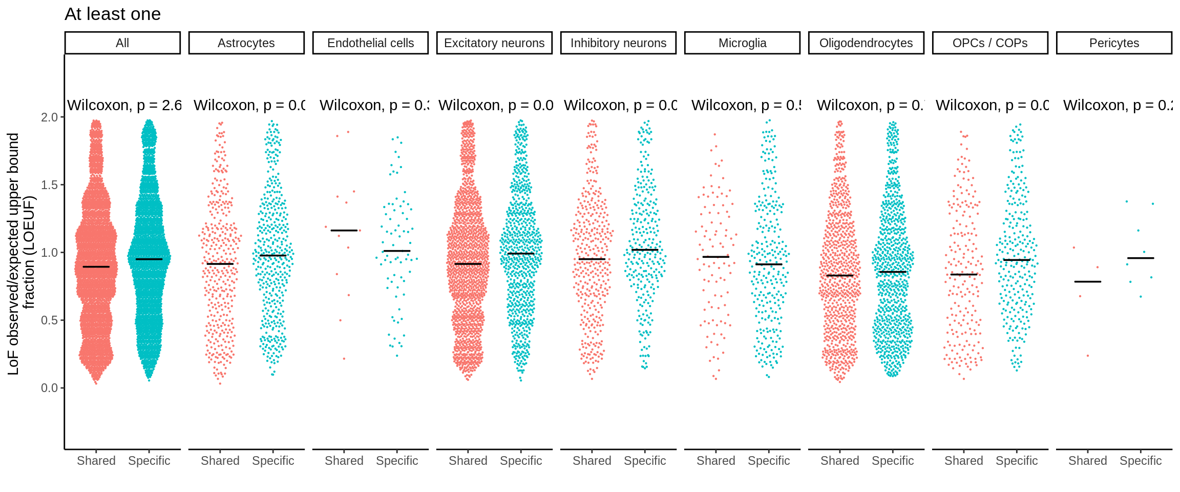
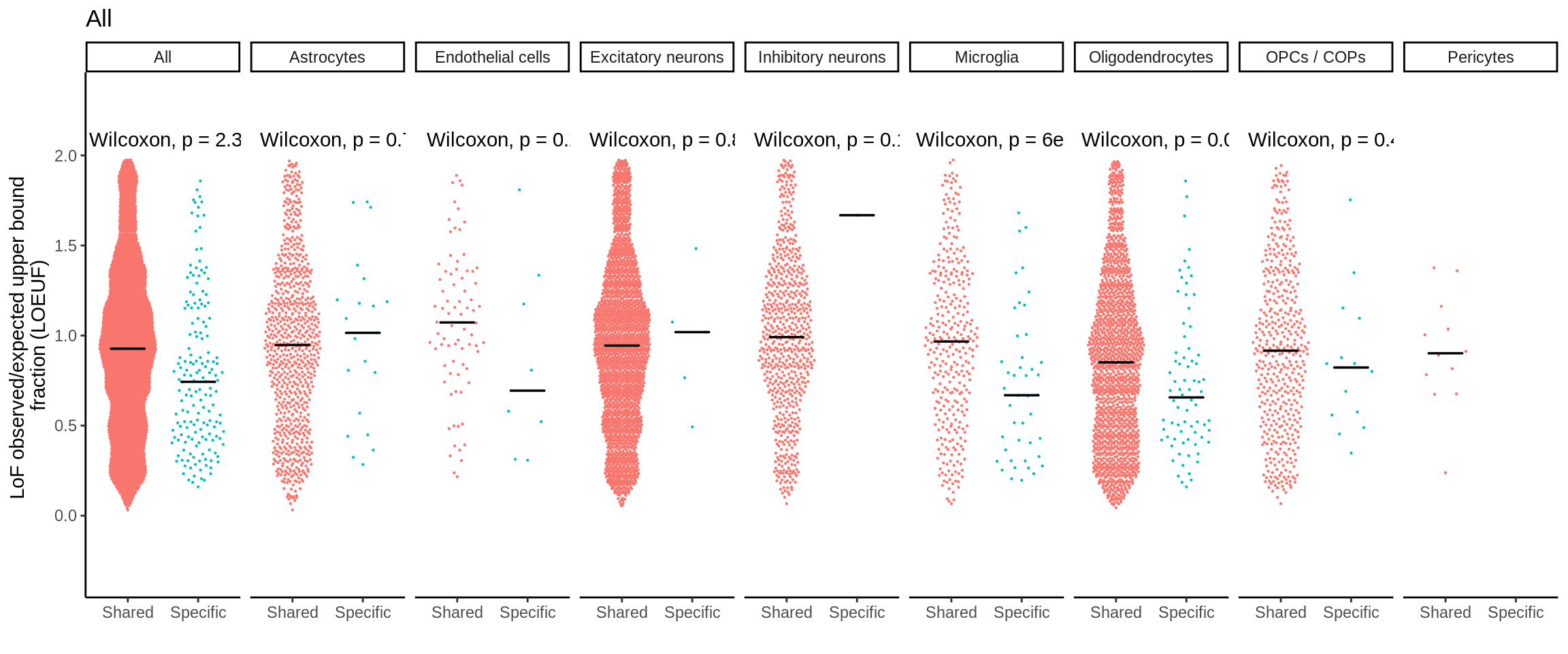
separate(gene_id,into=c('symbol','ensembl'),sep='_')d_short <- d_short %>% left_join(.,loeuf,by='ensembl')plot_loeuf_int <- function(test_var){
#Get only results from test variable (aggregate, at least one or all)
d_short_tmp <- d_short %>%
filter(test==test_var)
#Duplicate the data and set cell_type ids to All (all cell types)
d_short_all <- d_short_tmp %>%
mutate(cell_type_id='All')
d_short_plot <- rbind(d_short_tmp,d_short_all)
p <- d_short_plot %>%
ggplot(.,aes(specific,oe_lof_upper,col=specific)) +
ggbeeswarm::geom_quasirandom(size=0.1) +
ggpubr::stat_compare_means(vjust = -1) +
facet_wrap(~cell_type_id,nrow=1) +
theme_classic()+
stat_summary(fun = median,
fun.min = median,
fun.max = median,
geom = "crossbar",
width = 0.5,
size=0.25,
color='black') +
ylab("LoF observed/expected upper bound \nfraction (LOEUF)") +
theme(legend.position='none')+
scale_y_continuous(expand=c(0.25,0)) +
xlab('') +
ggtitle(test_var)
}p <- plot_loeuf_int('Aggregate')
ggsave(p,filename='output/figures/FigureS15A.png',width=17,height=3,dpi=300)
p
Past versions of unnamed-chunk-174-1.png
Version
Author
Date
865a38a
Julien Bryois
2022-02-10
p <- plot_loeuf_int('At least one')
ggsave(p,filename='output/figures/FigureS15B.png',width=17,height=3,dpi=300)
p
Past versions of unnamed-chunk-175-1.png
Version
Author
Date
865a38a
Julien Bryois
2022-02-10
p <- plot_loeuf_int('All')
ggsave(p,filename='output/figures/FigureS15C.png',width=17,height=3,dpi=300)
p
Past versions of unnamed-chunk-176-1.png
Version
Author
Date
865a38a
Julien Bryois
2022-02-10
Figure S18 - Number of coloc loci
coloc_ms <- read_tsv('output/coloc/coloc.ms.txt') %>% mutate(trait='Multiple Sclerosis')
coloc_ad <- read_tsv('output/coloc/coloc.ad.txt') %>% mutate(trait='Alzheimer')
coloc_scz <- read_tsv('output/coloc/coloc.scz.txt') %>% mutate(trait='Schizophrenia')
coloc_pd <- read_tsv('output/coloc/coloc.pd.txt') %>% mutate(trait='Parkinson')
coloc <- rbind(coloc_ms,coloc_ad,coloc_scz,coloc_pd) %>%
dplyr::select(symbol,trait,locus,PP.H4.abf)#Get all genes at GWAS loci in our study
gene_locus <- coloc %>% dplyr::select(locus,symbol,trait) %>% unique() #Get metabrain results
metabrain_s1 <- readxl::read_xlsx('data/metabrain/media-1.xlsx',skip=1,sheet = 2) %>%
mutate(disease=case_when(
outcome=="Alzheimer’s disease" ~ 'Alzheimer',
outcome=="Multiple sclerosis" ~ 'Multiple Sclerosis',
outcome=="Parkinson’s disease" ~ 'Parkinson',
outcome=="Schizophrenia" ~ 'Schizophrenia',
TRUE ~ outcome
)) %>%
dplyr::select(symbol=gene,trait=disease) %>%
filter(trait%in%c('Alzheimer','Multiple Sclerosis','Parkinson','Schizophrenia')) %>%
inner_join(.,gene_locus,by=c('symbol','trait'))New names:
* beta -> beta...3
* SE -> SE...4
* p -> p...5
* beta -> beta...7
* SE -> SE...8
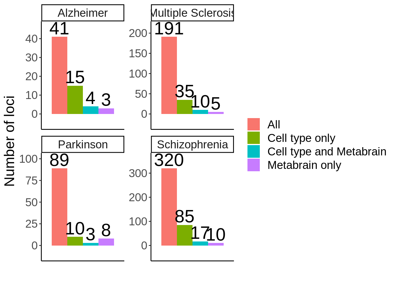
* ...coloc$locus_metabrain_sig <- coloc$locus%in%metabrain_s1$locusn_loci <- coloc %>%
mutate(locus_study_sig=ifelse(PP.H4.abf>0.7,TRUE,FALSE)) %>%
group_by(locus,trait) %>%
summarise(locus_metabrain_sig=any(locus_metabrain_sig),locus_study_sig=any(locus_study_sig)) %>%
ungroup() %>%
dplyr::count(trait,locus_metabrain_sig,locus_study_sig) %>%
mutate(label=factor(case_when(
locus_metabrain_sig & locus_study_sig ~ 'Cell type and Metabrain',
locus_metabrain_sig & !locus_study_sig ~ 'Metabrain only',
!locus_metabrain_sig & locus_study_sig ~ 'Cell type only',
!locus_metabrain_sig & !locus_study_sig ~ 'All'
),levels=c('All','Cell type only','Cell type and Metabrain','Metabrain only'))) %>%
dplyr::select(-locus_metabrain_sig,-locus_study_sig) %>%
group_by(trait) %>%
mutate(n=ifelse(label=='All',sum(n),n))`summarise()` regrouping output by 'locus' (override with `.groups` argument)p <- n_loci %>%
ggplot(.,aes(trait,n,fill=label)) + geom_col(position = position_dodge()) + facet_wrap(~trait,scales = 'free') + theme_classic() + theme(axis.ticks.x = element_blank(),axis.text.x = element_blank(),text=element_text(size=18),legend.title = element_blank()) + xlab('') +
ylab('Number of loci') + geom_text(aes(label=n),position = position_dodge(width=0.9),vjust=-0.2,size=8) +
scale_y_continuous(expand=c(0.2,0))
ggsave(p,filename = 'output/figures/FigureS18.png',width = 10,height = 6,dpi=300)
p
Past versions of unnamed-chunk-192-1.png
Version
Author
Date
865a38a
Julien Bryois
2022-02-10
Figure S19 - Exp of AD coloc genes
#Load AD coloc genes
coloc_ad <- read_tsv('output/coloc/coloc.ad.txt') %>%
  mutate(trait='Alzheimer') %>%
  filter(PP.H4.abf>=0.7)
#Load Pseudo-bulk
sum_expression_ms <- readRDS('data_sensitive/expression/ms_sum_expression.individual_id.rds') %>% mutate(dataset='ms')
sum_expression_ad <- readRDS('data_sensitive/expression/ad_sum_expression.individual_id.rds') %>% mutate(dataset='ad')#Let's merge the MS and AD dataset.
sum_expression <- rbind(sum_expression_ms,sum_expression_ad)#Get counts per million (CPM)
sum_expression <- sum_expression %>%
group_by(cell_type,individual_id) %>%
mutate(counts_scaled_1M=counts*10^6/sum(counts)) %>%
ungroup() %>%
as_tibble()#Keep AD coloc genes
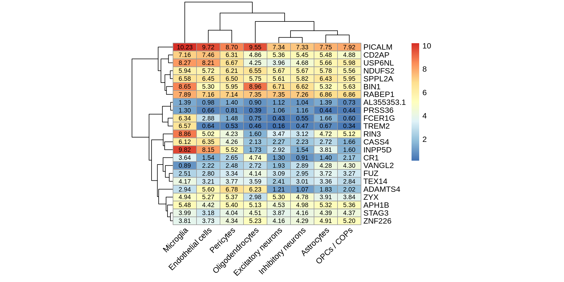
sum_expression <- sum_expression %>% filter(ensembl%in%coloc_ad$ensembl)m <- sum_expression %>%
group_by(cell_type,symbol) %>%
summarise(mean_cpm=mean(counts_scaled_1M,na.rm=TRUE)) %>%
ungroup() %>%
spread(cell_type,mean_cpm) %>%
column_to_rownames('symbol') %>%
as.matrix() pheatmap::pheatmap(log2(m+1),display_numbers = TRUE,number_color = 'black',angle_col = 45,cellwidth = 30,filename = 'output/figures/FigureS19.png',height = 5,width=7)pheatmap::pheatmap(log2(m+1),display_numbers = TRUE,number_color = 'black',angle_col = 45,cellwidth = 30)
Past versions of unnamed-chunk-200-1.png
Version
Author
Date
865a38a
Julien Bryois
2022-02-10
Figure S20 - GWAS enrichment
sum_expression_ms <- readRDS('data_sensitive/expression/ms_sum_expression.individual_id.rds') %>% mutate(dataset='ms')metadata <- read_tsv('data_sensitive/eqtl/covariate_pca_meta_fastqtl.txt') %>%
column_to_rownames('id') %>%
t() %>%
as.data.frame() %>%
rownames_to_column('individual_id') %>%
as_tibble() %>%
filter(study=='MS',diagnosis=='Ctrl')#Only keep controls
sum_expression_ms <- filter(sum_expression_ms,individual_id%in%metadata$individual_id)#Keep top 1k genes that were tested using magma
entrez_2_ensembl <- AnnotationDbi::toTable(org.Hs.eg.db::org.Hs.egENSEMBL) %>%
add_count(gene_id,name = 'n_entrez' ) %>%
add_count(ensembl_id,name='n_ensembl') %>%
filter(n_entrez==1,n_ensembl==1) %>%
dplyr::select(-n_entrez,-n_ensembl,GENE=gene_id,ensembl=ensembl_id)magma_genes <- read.table('data/gwas/ms/ms.annotated_35kbup_10_down.genes.out',header=TRUE) %>%
mutate(GENE=as.character(GENE)) %>%
inner_join(.,entrez_2_ensembl,by='GENE') %>%
dplyr::select(GENE,ensembl)sum_expression_ms <- sum_expression_ms %>%
group_by(cell_type,individual_id) %>%
mutate(libsize=sum(counts)) %>%
mutate(cpm=counts*10^6/libsize) %>%
ungroup() %>%
group_by(cell_type,symbol,ensembl) %>%
summarise(mean_cpm=mean(cpm)) %>%
group_by(symbol,ensembl) %>%
mutate(spe=mean_cpm/sum(mean_cpm)) %>%
ungroup() %>%
inner_join(.,magma_genes,by='ensembl') %>%
filter(mean_cpm>1) %>%
group_by(cell_type) %>%
slice_max(order_by = spe,n=1000) %>%
dplyr::select(cell_type,GENE) %>%
mutate(cell_type=make.names(cell_type)) %>%
write_tsv('data/magma_specific_genes/top1k.txt')source ~/.bashrc
cd data/magma_specific_genes
#Gene sets
top10k='top1k.txt'
#GWAS
ms='../gwas/ms/ms.annotated_35kbup_10_down.genes.raw'
ad='../gwas/ad/ad.annotated_35kbup_10_down.genes.raw'
pd='../gwas/pd/parkinsonMeta2020.annotated_35kbup_10_down.genes.raw'
scz='../gwas/scz/scz3.annotated_35kbup_10_down.genes.raw'
#Run MAGMA
magma --gene-results $ms --set-annot $top10k col=2,1 --out ms
magma --gene-results $ad --set-annot $top10k col=2,1 --out ad
magma --gene-results $pd --set-annot $top10k col=2,1 --out pd
magma --gene-results $scz --set-annot $top10k col=2,1 --out sczfiles <- list.files('data/magma_specific_genes',pattern='.gsa.out',full.names = T)d <- tibble(files=files) %>% mutate(file_content=map(files,read.table,header=TRUE)) %>%
mutate(disease=basename(files) %>% gsub('.gsa.out','',.)) %>%
dplyr::select(-files) %>%
unnest(file_content) %>%
mutate(gene_set=gsub('\\.',' ',VARIABLE) %>% gsub('OPCs COPs','OPCs / COPs',.)) %>%
group_by(disease) %>%
mutate(fdr.local=p.adjust(P,method='fdr')) %>%
mutate(sig=ifelse(fdr.local<=0.05,'<5%FDR','Not significant')) %>%
mutate(disease=case_when(
disease=='ad' ~ "Alzheimer's disease",
disease=='ms' ~ 'Multiple sclerosis',
disease=='pd' ~ "Parkinson's disease",
disease=='scz' ~ 'Schizophrenia'
))reorder_within <- function(x, by, within, fun = mean, sep = "___", ...) {
new_x <- paste(x, within, sep = sep)
stats::reorder(new_x, by, FUN = fun)
}
scale_x_reordered <- function(..., sep = "___") {
reg <- paste0(sep, ".+$")
ggplot2::scale_x_discrete(labels = function(x) gsub(reg, "", x), ...)
}
scale_y_reordered <- function(..., sep = "___") {
reg <- paste0(sep, ".+$")
ggplot2::scale_y_discrete(labels = function(x) gsub(reg, "", x), ...)
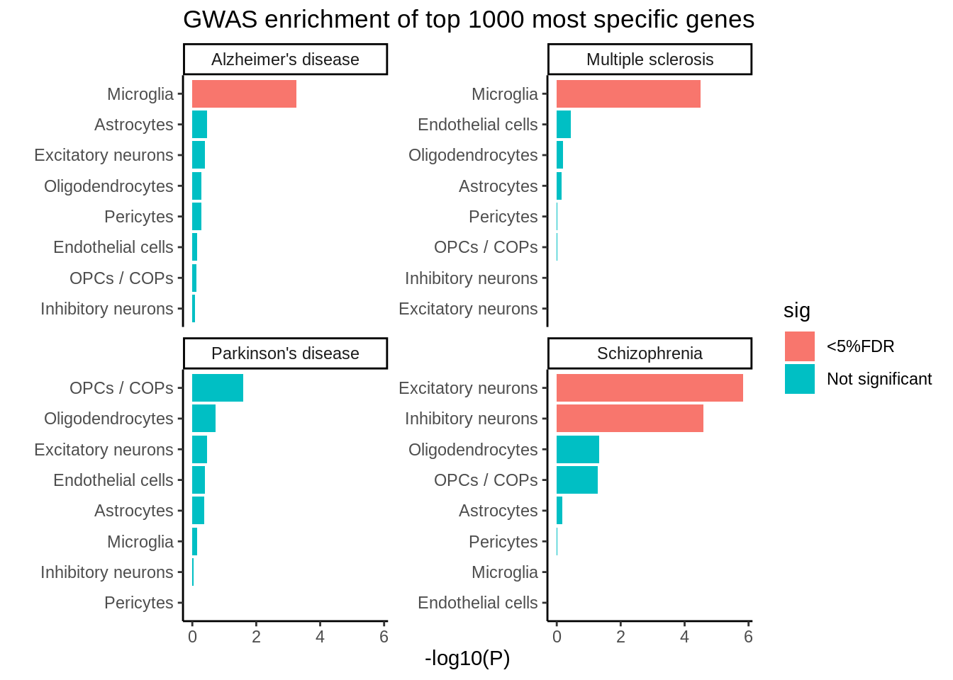
}p <- ggplot(d,aes(reorder_within(gene_set,-log10(P),disease),-log10(P),fill=sig)) +
geom_col(position = position_dodge()) +
coord_flip() +
facet_wrap(~disease,scales = 'free_y') +
theme_classic() + xlab('') +
scale_x_reordered() +
ggtitle('GWAS enrichment of top 1000 most specific genes')
p
Past versions of unnamed-chunk-211-1.png
Version
Author
Date
865a38a
Julien Bryois
2022-02-10
ggsave(p,filename='output/figures/FigureS20.png',width=8,height=5,dpi=300)
Figure S21 - Coloc MS GTEx and DICE
coloc_heatmap <- function(file,threshold=0.7,width=7,height=5,out_name){

  coloc_all <- read_tsv(file)

  #Get best coloc if same gene in same cell type was tested in two different loci
  coloc_all <- coloc_all %>% group_by(ensembl,tissue) %>%
    slice_max(n=1,order_by=PP.H4.abf,with_ties=FALSE) %>%
    ungroup()

  #Get best coloc if same symbol in same cell type was tested multiple times (different ensembl name for same symbol at same locus)
  coloc_all <- coloc_all %>% group_by(symbol,tissue) %>%
    slice_max(n=1,order_by=PP.H4.abf,with_ties=FALSE) %>%
    ungroup()

  #Get absolute value of effect size of the GWAS
  coloc_all <- mutate(coloc_all,beta=abs(beta_top_GWAS))

  coloc_all_matrix <- dplyr::select(coloc_all,tissue,symbol,PP.H4.abf) %>%
  filter(!is.na(symbol)) %>%
  unique() %>%
  spread(tissue,PP.H4.abf,fill=0) %>%
  column_to_rownames('symbol')

  coloc_all_format_per_gene <- coloc_all %>%
    group_by(ensembl) %>%
    filter(PP.H4.abf==max(PP.H4.abf),PP.H4.abf>threshold) %>%
    mutate(closest_gene=gsub('ENSG.+ - | - ENSG.+','',closest_gene)) %>% #Remove ENSEMBL name if a symbol + and ensembl gene name
                                                    #are both at same distance from GWAS top pick
    ungroup() %>%
    dplyr::rename(symbol_coloc=symbol) %>%
    filter(!is.na(symbol_coloc)) %>%
    arrange(-PP.H4.abf) %>%
    mutate(risk=case_when(
      direction ==1 ~ 'Up',
      direction ==-1 ~ 'Down',
      direction ==0 ~ 'Isoform'
    )) %>%
    column_to_rownames('symbol_coloc') %>%
    dplyr::rename(LOEUF=oe_lof_upper_bin)

  coloc_all_matrix_subset <- coloc_all_matrix[apply(coloc_all_matrix,1,function(x) any(x>threshold)),] %>% as.matrix()

  coloc_all_format_per_gene_direction <- coloc_all_format_per_gene[rownames(coloc_all_matrix_subset),] %>%
    dplyr::select(closest_gene,risk,LOEUF,beta)

 ha = HeatmapAnnotation(df = coloc_all_format_per_gene_direction[,2:3,drop=FALSE],
                         which ='row',
                         col = list('risk' = c("Up"="#E31A1C","Down"="#1F78B4","Isoform"="darkorange"),
                                    'LOEUF' = circlize::colorRamp2(c(0,10),c('white','springgreen4'))),
                         show_annotation_name = c('risk' = TRUE,'LOEUF'=TRUE),
                         annotation_name_rot = 45
                         )

  hb = HeatmapAnnotation(df = coloc_all_format_per_gene_direction[,4,drop=FALSE],
                         which ='row',
                         col = list(circlize::colorRamp2(c(min(coloc_all_format_per_gene_direction[[4]],na.rm=T),
                                                                  max(coloc_all_format_per_gene_direction[[4]],na.rm=T)),c('white','palevioletred3'))) %>%
                           setNames(colnames(coloc_all_format_per_gene_direction)[4]),
                         annotation_name_rot = 45
                         )

   ht <- Heatmap(coloc_all_matrix_subset,col=viridis(100),
                right_annotation=ha,column_names_rot = 45,
                left_annotation = hb,
                #row_names_side = 'left',
                #row_dend_side = 'right',
                row_split = coloc_all_format_per_gene_direction[, 1],
                row_title_rot = 0,
                cluster_rows = FALSE,
                layer_fun = function(j, i, x, y, width, height, fill) {
                                          grid.text(sprintf("%.2f", pindex(coloc_all_matrix_subset, i, j)),
                                                    x, y, gp = gpar(fontsize = 10,col="black"))
                                                      },
                #row_title_gp = gpar(col = 'red', font = 2),
                #row_title = rep('',length(unique(coloc_all_format_per_gene_direction[, 1]))),
                heatmap_legend_param = list(title="PP",at = c(0,0.5,1),
                                            lables = c(0,0.5,1)))


  pdf(out_name,width = width,height=height)
  draw(ht,heatmap_legend_side = "right")
  dev.off()

  return(ht)
}
coloc_heatmap('output/coloc/coloc.ms.gtex_dice.txt',threshold=0.7,height=30,width=10,out_name='output/figures/FigureS21.pdf')
Figure S23 - PCs
From expression data
sum_expression_ms <- readRDS('data_sensitive/expression/ms_sum_expression.individual_id.rds') %>% mutate(dataset='ms')
sum_expression_ad <- readRDS('data_sensitive/expression/ad_sum_expression.individual_id.rds') %>% mutate(dataset='ad')
sum_expression <- rbind(sum_expression_ms,sum_expression_ad)
Get number of cells and total counts (log)
exp_info <- sum_expression %>%
  group_by(cell_type,individual_id) %>%
  summarise(log_tot_counts=log(sum(counts)+1),
            n_cells=unique(n_cells)) %>%
  ungroup()
`summarise()` regrouping output by 'cell_type' (override with `.groups` argument)ad_meta <- read_tsv('data_sensitive/expression/sample_individual_ad.txt') %>%
group_by(individual_id) %>%
summarise(n_samples_per_id=n(),
tissue=paste0(tissue,collapse=','),
age=unique(age),
post_mortem_m=unique(post_mortem_m),
sex=unique(sex))Parsed with column specification:
cols(
sample_id = col_character(),
individual_id = col_character(),
age = col_double(),
post_mortem_m = col_double(),
sex = col_character(),
tissue = col_character()
)`summarise()` ungrouping output (override with `.groups` argument)ms_meta <- read_tsv('data_sensitive/expression/sample_individual_ms.txt') %>%
group_by(individual_id) %>%
summarise(n_samples_per_id=n(),
tissue=paste0(unique(tissue),collapse=','),
age=unique(age),
post_mortem_m=unique(post_mortem_m),
sex=unique(sex))Parsed with column specification:
cols(
sample_id = col_character(),
individual_id = col_character(),
age = col_double(),
post_mortem_m = col_double(),
sex = col_character(),
tissue = col_character()
)`summarise()` regrouping output by 'individual_id' (override with `.groups` argument)meta <- rbind(ad_meta,ms_meta) %>%
mutate(tissue=case_when(
tissue=='GM' ~ 'Cortex',
tissue=='WM' ~ 'Deep white matter',
tissue=='GM,WM' ~ 'Cortex,Deep white matter',
tissue=='Prefrontal cortex' ~ 'Cortex',
tissue=='Deep white matter,Prefrontal cortex' ~ 'Cortex,Deep white matter',
tissue=='Deep white matter,Temporal cortex' ~ 'Cortex,Deep white matter',
TRUE ~ tissue
))pc_files <- list.files('data_sensitive/eqtl/PC70/',pattern='.cov.txt.gz',full.names = TRUE)get_pc_var_assoc <- function(i){
message(i)
#Read covariate file, add expression related metadata and metadata
d <- read_tsv(pc_files[i]) %>%
t() %>%
as.data.frame() %>%
rownames_to_column() %>%
setNames(.[1,]) %>%
dplyr::slice(2:n()) %>%
dplyr::rename(individual_id=id) %>%
mutate(cell_type=basename(pc_files[i]) %>% gsub('.cov.txt.gz','',.) %>% gsub('\\.',' ',.) %>% gsub('OPCs COPs','OPCs / COPs',.)) %>%
mutate(across(contains('PC'),as.numeric)) %>%
left_join(.,exp_info,by=c('individual_id','cell_type')) %>%
left_join(.,meta,by='individual_id') %>%
as_tibble() %>%
dplyr::rename(PC1_genotype=PC1,
PC2_genotype=PC2,
PC3_genotype=PC3)
#Compute correlation between numerical variables and expression PCs
num <- dplyr::select(d,PC1_genotype,PC2_genotype,PC3_genotype,log_tot_counts,n_cells,n_samples_per_id,age,post_mortem_m,PC1_exp:PC70_exp) %>%
gather(x_var,x_val,PC1_genotype:post_mortem_m) %>%
gather(y_var,y_val,PC1_exp:PC70_exp) %>%
group_by(x_var,y_var) %>%
summarise(pvalue=cor.test(x_val,y_val)$p.value) %>%
arrange(pvalue)
#Compute linear regression for factors
fact <- dplyr::select(d,study,diagnosis,tissue,sex,PC1_exp:PC70_exp) %>%
gather(x_var,x_val,study:sex) %>%
gather(y_var,y_val,PC1_exp:PC70_exp) %>%
group_by(x_var,y_var) %>%
summarise(pvalue = anova(lm(y_val~1), lm(y_val~x_val))$`Pr(>F)`[2]) %>%
arrange(pvalue)
#get results
res <- rbind(num,fact) %>%
mutate(p_adj=p.adjust(pvalue,method='fdr')) %>%
arrange(p_adj) %>%
mutate(sig=ifelse(p_adj<0.05,'5% FDR','Not significant')) %>%
group_by(y_var) %>%
mutate(n_sig=sum(sig=='5% FDR')) %>%
filter(n_sig>0) %>%
mutate(exp_PC=gsub('PC','',y_var) %>% gsub('_exp','',.) %>% as.numeric()) %>%
arrange(exp_PC)
#set factor levels
lev <- res %>% dplyr::select(y_var,exp_PC) %>% unique()
res <- mutate(res,y_var=factor(y_var,levels=lev$y_var))
#set cell type tested
res <- res %>% mutate(cell_type=unique(d$cell_type))
return(res)
}pc_res <- lapply(1:length(pc_files),get_pc_var_assoc) %>%
bind_rows()1Parsed with column specification:
cols(
.default = col_character()
)See spec(...) for full column specifications.`summarise()` regrouping output by 'x_var' (override with `.groups` argument)
`summarise()` regrouping output by 'x_var' (override with `.groups` argument)2Parsed with column specification:
cols(
.default = col_character()
)See spec(...) for full column specifications.`summarise()` regrouping output by 'x_var' (override with `.groups` argument)
`summarise()` regrouping output by 'x_var' (override with `.groups` argument)3Parsed with column specification:
cols(
.default = col_character()
)See spec(...) for full column specifications.`summarise()` regrouping output by 'x_var' (override with `.groups` argument)
`summarise()` regrouping output by 'x_var' (override with `.groups` argument)4Parsed with column specification:
cols(
.default = col_character()
)See spec(...) for full column specifications.`summarise()` regrouping output by 'x_var' (override with `.groups` argument)
`summarise()` regrouping output by 'x_var' (override with `.groups` argument)5Parsed with column specification:
cols(
.default = col_character()
)See spec(...) for full column specifications.`summarise()` regrouping output by 'x_var' (override with `.groups` argument)
`summarise()` regrouping output by 'x_var' (override with `.groups` argument)6Parsed with column specification:
cols(
.default = col_character()
)See spec(...) for full column specifications.`summarise()` regrouping output by 'x_var' (override with `.groups` argument)
`summarise()` regrouping output by 'x_var' (override with `.groups` argument)7Parsed with column specification:
cols(
.default = col_character()
)See spec(...) for full column specifications.`summarise()` regrouping output by 'x_var' (override with `.groups` argument)
`summarise()` regrouping output by 'x_var' (override with `.groups` argument)8Parsed with column specification:
cols(
.default = col_character()
)See spec(...) for full column specifications.`summarise()` regrouping output by 'x_var' (override with `.groups` argument)
`summarise()` regrouping output by 'x_var' (override with `.groups` argument)px <- pc_res %>% filter(y_var%in%c('PC1_exp','PC2_exp','PC3_exp','PC4_exp','PC5_exp')) %>% ggplot(.,aes(-log10(pvalue),x_var,fill=sig)) +
geom_col() +
facet_grid(y_var~cell_type) +
theme_bw() +
ylab('') +
ggtitle('Association of technical covariates with expression PCs')#Plot of Astrocytes PCs vs top associated variables
i <- 1
d <- read_tsv(pc_files[i]) %>%
t() %>%
as.data.frame() %>%
rownames_to_column() %>%
setNames(.[1,]) %>%
dplyr::slice(2:n()) %>%
dplyr::rename(individual_id=id) %>%
mutate(cell_type=basename(pc_files[i]) %>% gsub('.cov.txt.gz','',.) %>% gsub('\\.',' ',.) %>% gsub('OPCs COPs','OPCs / COPs',.)) %>%
mutate(across(contains('PC'),as.numeric)) %>%
left_join(.,exp_info,by=c('individual_id','cell_type')) %>%
left_join(.,meta,by='individual_id') %>%
as_tibble() %>%
dplyr::rename(PC1_genotype=PC1,
PC2_genotype=PC2,
PC3_genotype=PC3)Parsed with column specification:
cols(
.default = col_character()
)See spec(...) for full column specifications.p1 <- ggplot(d,aes(PC1_exp,PC2_exp,col=study)) + geom_point() + theme_classic()
p2 <- ggplot(d,aes(PC1_exp,PC2_exp,col=tissue)) + geom_point() + theme_classic()
p3 <- ggplot(d,aes(PC1_exp,PC2_exp,col=PC1_genotype)) + geom_point() + theme_classic() + scale_color_viridis_c()
p4 <- ggplot(d,aes(PC1_exp,PC2_exp,col=diagnosis)) + geom_point() + theme_classic()py <- p1 + p2 + p3 + p4 + plot_annotation(title = 'Astrocytes') & xlab('PC1 expression') & ylab('PC2 expression')
p <- px +py + plot_layout(widths = c(2, 1))
ggsave(p,filename=paste0('output/figures/FigureS23.png'),width=24,height=8)
p
Past versions of unnamed-chunk-226-1.png
Version
Author
Date
865a38a
Julien Bryois
2022-02-10
Locuszoom
dir.create('data/locuszoom/',showWarnings = FALSE)ad_coloc <- read_tsv('output/coloc/coloc.ad.txt')Parsed with column specification:
cols(
.default = col_double(),
locus = col_character(),
closest_gene = col_character(),
GWAS_snp = col_character(),
GWAS_snp_pos = col_character(),
symbol = col_character(),
ensembl = col_character(),
tissue = col_character(),
type = col_character(),
coloc_method = col_character()
)See spec(...) for full column specifications.ad_gwas <- data.table::fread('data/gwas/ad/GCST90012877_buildGRCh37.tsv',data.table = FALSE) %>% as_tibble()get_locuszoom_input <- function(coloc,gwas,cell_type,symbol_selected){
locus <- coloc %>% filter(symbol==symbol_selected,tissue==cell_type) %>% pull(locus)
chr <- gsub(':.+','',locus) %>% gsub('chr','',.)
start <- gsub('chr.+:','',locus) %>% gsub('_.+','',.) %>% as.numeric()
end <- gsub('chr.+:','',locus) %>% gsub('.+_','',.) %>% as.numeric()
gwas_locus <- filter(gwas,chromosome==chr,
base_pair_location>=start & base_pair_location<=end) %>%
dplyr::select(variant_id,pvalue_gwas=p_value)
eqtl <- data.table::fread(paste0('data_sensitive/eqtl/PC70_nominal/',make.names(cell_type),'.',chr,'.gz'),data.table = FALSE) %>% as_tibble() %>%
separate(V1,into=c('symbol','ensembl'),sep='_') %>%
filter(symbol==symbol_selected) %>%
dplyr::select(variant_id=V2,pvalue_eqtl=V4)
out <- inner_join(gwas_locus,eqtl,by='variant_id')
write_tsv(out,path = paste0('data/locuszoom/',symbol_selected,'.',cell_type,'.txt'))
}get_locuszoom_input(ad_coloc,ad_gwas,'Microglia','INPP5D')
get_locuszoom_input(ad_coloc,ad_gwas,'Microglia','PICALM')
sessionInfo()R version 4.0.1 (2020-06-06)
Platform: x86_64-pc-linux-gnu (64-bit)
Running under: CentOS Linux 7 (Core)
Matrix products: default
BLAS/LAPACK: /pstore/apps/OpenBLAS/0.3.1-GCC-7.3.0-2.30/lib/libopenblasp-r0.3.1.so
locale:
[1] en_US.UTF-8
attached base packages:
[1] grid parallel stats4 stats graphics grDevices utils
[8] datasets methods base
other attached packages:
[1] rhdf5_2.32.4
[2] viridis_0.5.1
[3] viridisLite_0.3.0
[4] ComplexHeatmap_2.7.6.1002
[5] liftOver_1.12.0
[6] Homo.sapiens_1.3.1
[7] TxDb.Hsapiens.UCSC.hg19.knownGene_3.2.2
[8] org.Hs.eg.db_3.11.4
[9] GO.db_3.11.4
[10] OrganismDbi_1.30.0
[11] GenomicFeatures_1.40.0
[12] AnnotationDbi_1.50.0
[13] Biobase_2.48.0
[14] rtracklayer_1.48.0
[15] GenomicRanges_1.40.0
[16] GenomeInfoDb_1.24.0
[17] IRanges_2.22.2
[18] S4Vectors_0.26.1
[19] BiocGenerics_0.34.0
[20] gwascat_2.20.1
[21] scales_1.1.1
[22] patchwork_1.0.0
[23] qvalue_2.20.0
[24] forcats_0.5.0
[25] stringr_1.4.0
[26] dplyr_1.0.0
[27] purrr_0.3.4
[28] readr_1.3.1
[29] tidyr_1.1.0
[30] tibble_3.0.1
[31] ggplot2_3.3.3
[32] tidyverse_1.3.0
[33] workflowr_1.6.2
loaded via a namespace (and not attached):
[1] R.utils_2.9.2 tidyselect_1.1.0
[3] htmlwidgets_1.5.1 RSQLite_2.2.0
[5] BiocParallel_1.22.0 munsell_0.5.0
[7] withr_2.2.0 colorspace_1.4-1
[9] knitr_1.28 rstudioapi_0.11
[11] ggsignif_0.6.0 labeling_0.3
[13] git2r_0.27.1 GenomeInfoDbData_1.2.3
[15] bit64_0.9-7 farver_2.0.3
[17] pheatmap_1.0.12 rprojroot_1.3-2
[19] vctrs_0.3.1 generics_0.0.2
[21] xfun_0.14 BiocFileCache_1.12.0
[23] R6_2.4.1 ggbeeswarm_0.6.0
[25] clue_0.3-57 bitops_1.0-6
[27] DelayedArray_0.14.0 assertthat_0.2.1
[29] promises_1.1.1 nnet_7.3-14
[31] beeswarm_0.2.3 gtable_0.3.0
[33] Cairo_1.5-12.2 rlang_0.4.10
[35] GlobalOptions_0.1.2 splines_4.0.1
[37] rstatix_0.6.0 acepack_1.4.1
[39] checkmate_2.0.0 broom_0.5.6
[41] BiocManager_1.30.10 yaml_2.2.1
[43] reshape2_1.4.4 abind_1.4-5
[45] modelr_0.1.8 backports_1.1.7
[47] httpuv_1.5.4 Hmisc_4.4-0
[49] RBGL_1.64.0 tools_4.0.1
[51] ellipsis_0.3.1 RColorBrewer_1.1-2
[53] Rcpp_1.0.6 plyr_1.8.6
[55] base64enc_0.1-3 progress_1.2.2
[57] zlibbioc_1.34.0 RCurl_1.98-1.2
[59] prettyunits_1.1.1 ggpubr_0.4.0
[61] rpart_4.1-15 openssl_1.4.1
[63] GetoptLong_1.0.5 SummarizedExperiment_1.18.1
[65] haven_2.3.1 ggrepel_0.8.2
[67] cluster_2.1.0 fs_1.4.1
[69] magrittr_1.5 data.table_1.12.8
[71] openxlsx_4.1.5 circlize_0.4.12
[73] reprex_0.3.0 whisker_0.4
[75] matrixStats_0.56.0 hms_0.5.3
[77] evaluate_0.14 XML_3.99-0.3
[79] rio_0.5.16 jpeg_0.1-8.1
[81] readxl_1.3.1 gridExtra_2.3
[83] shape_1.4.5 compiler_4.0.1
[85] biomaRt_2.44.4 crayon_1.3.4
[87] R.oo_1.23.0 htmltools_0.5.1.1
[89] later_1.1.0.1 Formula_1.2-3
[91] lubridate_1.7.9 DBI_1.1.0
[93] dbplyr_1.4.4 rappdirs_0.3.1
[95] Matrix_1.2-18 car_3.0-8
[97] cli_2.0.2 R.methodsS3_1.8.0
[99] pkgconfig_2.0.3 GenomicAlignments_1.24.0
[101] foreign_0.8-80 xml2_1.3.2
[103] vipor_0.4.5 XVector_0.28.0
[105] rvest_0.3.5 digest_0.6.25
[107] graph_1.66.0 Biostrings_2.56.0
[109] rmarkdown_2.2 cellranger_1.1.0
[111] htmlTable_1.13.3 curl_4.3
[113] Rsamtools_2.4.0 rjson_0.2.20
[115] lifecycle_0.2.0 nlme_3.1-148
[117] jsonlite_1.6.1 Rhdf5lib_1.10.0
[119] carData_3.0-4 askpass_1.1
[121] fansi_0.4.1 pillar_1.4.4
[123] lattice_0.20-41 httr_1.4.1
[125] survival_3.1-12 glue_1.4.1
[127] zip_2.0.4 png_0.1-7
[129] bit_1.1-15.2 stringi_1.4.6
[131] blob_1.2.1 latticeExtra_0.6-29
[133] memoise_1.1.0